Textbook: Peter Atkins, Julio de Paula - Physical Chemistry for the Life Sciences
Table of Contents:
| Section # | Topic | Chapter |
|---|---|---|
| 1. | Microscopic systems and quantization | 9.1-9.4 |
| 2. | Spartan I: Introduction to Spartan | 10.9 |
| 3. | Spartan II: Particle in a Box (PIB) - Polyenes | 9.1-9.4; 10.9 |
| 4. | Literature Review (Juffmann) | - |
| 5. | Spartan III: Harmonic Oscillator | 9.6-9.8 |
| 6. | Midterm Review #1 | 9-11 |
| 7. | Spartan IV: PES of H2 & Peptide backbone dihedral scan | 10.9; 11.13; 11.17 |
| 8. | Chimera I: Getting familiar with X-ray and NMR structures (MDM2) | 11.3-11.4 |
| 9. | Chimera II: Calculating ∆SASA | - |
| 10. | HW Review | 11 & 12 |
| 11. | Midterm Review #2 | 1; 11; 12 |
| 12. | Simbiology I: binding reactions | 12 |
| Chemical Kinetics I: Python version | ||
| 13. | Simbiology II: folding intermediates | 12 |
| Chemical Kinetics II: Python version | ||
| 14. | Review for Final | - |
| 15. | Extra | - |
1.
1. To what speed must a proton be accelerated for it to have a wavelength of 3.0 cm?
Keywords: proton, wavelength, speed
In 1923 de Broglie says that matter has wave-like properties:
$$ \lambda = \frac{h}{p}, $$where $h$ is Plancks constant ($6.626x10^{-34} Js$). From classical mechanics we know linear momentum is the product of mass and velocity ($ p = mv $). Then, we solve for velocity:
$$ v = \frac{h}{\lambda\space m_{proton}} = 1.3 x 10^{-5} \text{m }s^{-1}$$2. Calculate the energy per mole of photons for radiation of wavelength (a) 200 nm (ultraviolet), (b) 150 pm (X-ray), (c) 1.00 cm (microwave).
In 1900 Bohr and Planck determined that energy is quantized (discrete energy levels).
$$ E = nh\nu, $$where $c = \lambda \nu$ and $n$ is the number of photons ($6.022x10^{23} photons/mole$).
Then,
$$ E = nh \frac{c}{\lambda}$$Therefore,
$E =$ (a) $5.97x10^{5} J$, (a) $7.95x10^{8} J$, (a) $11.6 J$
3. The work function for metallic rubidium is 2.09 eV. Calculate the kinetic energy and the speed of the electrons ejected by light of wavelength (a) 650 nm, (b) 195 nm.
Einstein published the a paper on the photoelectric effect in 1905 (won Nobel Prize in 1921). The main idea is conservation of energy: $$E_{total} = V + E_{k} $$
Here, $V = \phi \equiv \text{Work Function}$, $E_{total} = h\nu$ and $ E_{k} = \frac{1}{2}mv^{2}$. The work function, $\phi$ is defined as the amount of energy required to eject an electron, which is also known as ionization energy.
$$h\nu = \phi + \frac{1}{2}m_{e}v^{2},$$where $m_{e}$ is the mass of an electron ($9.11*10^{-31} kg$).

To calculate kinetic energy, we rearrange for $E_{k}$ to obtain
$$E_{k} = \frac{1}{2}m_{e}v^{2} = \phi - h\nu $$Solving for velocity gives:
$$ v = \sqrt{\frac{2}{m_{e}}(\frac{hc}{\lambda} - \phi)} = \sqrt{\frac{2}{m_{e}}E_{k}}$$Therefore,
For $\lambda = 650 nm$, $E_{k} = -3.00 x 10^{-20} J$, which means the amount of energy is insufficient to eject the electron and $v = 0 m/s$.
Side notes:
Ionization energy and electron affinity increase as your go $\uparrow$ and $\rightarrow$
Ionization energies are always positive values.
9.18 An electron is confined to a linear region with a length of the same order as the diameter of an atom (about 100 pm). Calculate the minimum uncertainties in its position and speed.
In 1927 Werner Heisenberg devised one of the postulates of quantum mechanics called Heisenberg's Uncertainty Principle. This postulate states that complementary observables cannot be measured with absolute certainty i.e., if the position of a particle is certain, then its momentum is uncertain and visa-versa.
$$\Delta x \Delta p \underline{>} \frac{h}{4\pi} $$We can say that the minimum uncertainty in position is 100 pm, which is $1.0 x 10^{-10} m$. Now, we need to find the minimum uncertainty in speed. Substituting for $\Delta p = m_{e} \Delta v$ ($m_{e} = 9.11x10^{-31}kg$) into the inequality above gives
$$ \Delta p = m_{e} \Delta v \underline{>} \frac{h}{4\pi \Delta x } \implies \Delta v \underline{>} \frac{h}{4\pi \Delta x \space m_{e}}$$Therefore,
$$\Delta v \underline{>} 5.78x10^{5} m/s$$Jump to table of contents.
1-D time-independent $Schr\ddot{o}dinger$ Equation & 1-D Particle in a Box
The wavefunction, $\psi(x)$
$$ \psi(x) = Asin(\frac{n\pi x}{L}) $$Time-Independent $Schr\ddot{o}dinger$ Equation
$$\hat{H}\psi(x) = E\psi(x)$$$$ \text{Operator $\space f^{\underline{n}}$ = Eigenvalue $\space f^{\underline{n}}$} $$Hamiltonian Operator in 1-D
$$ \hat{H} = -\frac{\hbar^{2}}{2m}(\frac{\partial^{2}}{\partial x^{2}}) + V(x)$$Let the kinetic energy and the potential energy be defined as the following:
$$ E_{k} = \frac{1}{2}mv^{2} = \frac{\hat{p}^{2}}{2m} = -\frac{\hbar^{2}}{2m}(\frac{\partial^{2}}{\partial x^{2}}),$$and Hooke's law (springs) will define the potential energy of our bonds.
$$F = -K_{f}x,$$where $ F = -\frac{dV(X)}{dx} \implies Fdx = dV(x)$
$$ \int Fdx = \int -K_{f}xdx = \int dV(x) $$$$ V(x) = \frac{1}{2}k_{f}x^{2} $$Recall:

Now we will operate on the wavefunction, $\psi(x)$
Now, consider a 1-dimensional (x) box of length, L. The particle has a free path and no potential energy inside the box, but infinite potential energy outside the box.

we need to plug $Asin(n\pi x/L)$ in for $\psi(x)$ and solve. Note that if we take the derivative of $sin(x)$ with respect to x two times, we get back a -$sin(x)$. This is called an eigenfunction of the $\frac{\partial^{2}}{\partial x^{2}}$ operator because we get back the function sin(x).
Okay, so we let $\psi(x) = Asin(\frac{n\pi x}{L})$ and say:
$$\hat{H}\psi(x) = E\psi(x)$$$$ \hat{H}\psi(x)\hspace{0.5cm} = \hspace{0.5cm} -\frac{\hbar^{2}}{2m}(\frac{\partial^{2} Asin(\frac{n\pi x}{L})}{\partial x^{2}})\hspace{0.5cm},$$where $\hbar = h/(2\pi)$ and we know that
$$(\frac{\partial^{2} Asin(\frac{n\pi x}{L})}{\partial x^{2}}) = -\frac{n^{2}}{L^{2}}Asin(\frac{n\pi x}{L}) $$Then,
$$ E\psi(x) = \frac{h^{2}n^{2}}{8mL^{2}} Asin(\frac{n\pi x}{L}) \implies E = \frac{h^{2}n^{2}}{8mL^{2}}$$Particle in a Box (PIB)
where the # of nodes = n-1, and the wavelength is $2\times L/n$, the length of the box.
$$ \lambda = \frac{2L}{n} $$Jump to table of contents.
2.
Computer lab #1 – Intro to Spartan
Goal: The goal of this exercise is to familiarize yourself with Spartan, and the kind of information you can get using it.
Introduction
In class, we have been discussing wavefunction solutions $\psi(x)$ to Schrödinger’s Equation, $H\psi = E\psi$, for an electron as a function of its position $x$. Computational chemistry programs approximate solutions to Schrödinger Equation, but for multi-electron systems—atoms and molecules:
$$\hat{H}\psi(x_{1}, x_{2},…x_{n}) = E\psi(x_{1}, x_{2},…x_{n}).$$It turns out that if you assume the electrons do not interact (i.e. do not feel each others’ repulsion), then the wave function is separable, i.e. solutions are products of one-electron wavefunctions $\psi(x_{1}, x_{2},…x_{n}) = \psi_{1}(x_{1}) \psi_{2}(x_{2})… \psi_{n}(x_{n})$. The $\psi_{i}$ are called orbitals.
Quantum chemistry methods try to solve for $\psi$ as a product of orbitals, with different ways of approximating the effects of electron interaction. The computed solution is a set of molecular orbitals (MOs), each a one-electron wavefunction that can be spread out over the entire molecule.
As you might imagine, MOs are complicated entities, but can be represented as a superposition (i.e. a sum) of atomic orbitals (AOs), i.e. wavefunctions of electrons bound to a specific nucleus. For reasons of computational efficiency, each AO in turn is (usually) represented by superposition of simpler functions called basis functions. The more basis functions you use, the better the approximation, but at increased computational cost.
In this lab we will explore the effects of using different basis sets (i.e. groups of basis functions) for an atomic orbital calculation. We will consider three different basis sets, STO-3G, 3-21G, and 6-31G* (Figure 1).
Introduction to Hartree Fock and Basis Sets:
Hartree Fock method
- approximation (variational approach) for the determination of $\Psi$ and $E$ of a quantum many-body system in a stationary state
This does a iterative search for $\psi$ where $E'$ is smallest compared to the actual E.
$$E'=\int \Psi^{*} H\Psi d\tau = <\Psi^{*}|H|\Psi>$$$$E'=\int \Psi^{*} E\Psi d\tau = E \int \Psi^{*}\Psi = E$$$$E′ > E$$Slater-Type Orbitals (STO’s)
Abbreviation: STO-nG, where n is an integer that represents the number of primitive Gaussian functions within a single basis function.
- minimal basis set (cheaper computationally)
For example, consider oxygen’s electronic configuration $1s^2 2s^2 2p^4$. We represent molecular orbitals (MOs) as a superposition of atomic orbitals (AOs):
$$\mathbf \Psi_{STO-3G}= \sum_{i}^{m} C_i\psi_{(STO-3G)}(i) = C_1\psi_{STO-3G}(1s) + C_2\psi_{STO-3G}(2s) + C_3\psi_{STO-3G}(2p_{x}) + C_4\psi_{STO-3G}(2p_{y}) + C_5\psi_{STO-3G}(2p_{z}),$$where $n$ primitive Gaussian orbitals are fitted to a single Slater-type orbital (STO). The core and valence orbitals are represented by the same number of primitive Gaussian functions $\mathbf \phi_i$. For example, an STO-3G basis set for the 1s, 2s and 2p orbital of the carbon atom are all linear combination of 3 primitive Gaussian functions. For example, a STO-3G s orbital is given by:
$$\mathbf \psi_{STO-3G}(s)= \sum_{i}^{n} c_i\phi_i = c_1\phi_1 + c_2\phi_2 + c_3\phi_3 ,$$where
$$\mathbf \phi_1 = \left (\frac{2\alpha_1}{\pi} \right ) ^{3/4}e^{-\alpha_1 r^2}$$$$\mathbf \phi_2 = \left (\frac{2\alpha_2}{\pi} \right ) ^{3/4}e^{-\alpha_2 r^2}$$$$\mathbf \phi_3 = \left (\frac{2\alpha_3}{\pi} \right ) ^{3/4}e^{-\alpha_3 r^2}$$The $\alpha_i$'s and $c_i$'s are tabulated values for each element and contained in a library within Spartan. The $C_{i}$'s are what is changing iteratively.
For singlet, the method treats electrons as indistinguishable (2 electrons in an orbital are not labeled). For triplet, the method labels α and β electrons to 2 electrons in an orbital (convention is to start from α as the lowest energy one).
6-31G the core orbital is a CGTO made of 6 Gaussians, and the valence is described by two orbitals — one CGTO made of 3 Gaussians, and one single Gaussian.
6-31G* [or 6-31G(d)] is 6-31G with added d polarization functions on non-hydrogen atoms.
Jump to table of contents.
Directions:
Login to your account by using your tuid and password.
Open Spartan by clicking on its icon on the desktop.
File > New Build (or click icon on upper left)
Build an oxygen atom:
Select oxygen from panel and click anywhere in main window.
Remove bonds by using delete tool (build > delete, or select eraser icon in the panel. You have to click it each time you want to delete an atom)
Setup > Calculations… Parameters:
Energy at ground state
With Hartree-Fock STO-3G in vacuum, total charge: neutral, zero unpaired electrons
Check box for orbital and energy
Check box for charges and bond orders
Submit (it will ask you where to save the data, it is good to give them proper names and save them on Desktop).
Wait until calculation is done (a few seconds).
Display > orbital energies
- Record approximate HOMO and LUMO energies (click on spectrum to get values)
Display > Surfaces:
Add HOMO, LUMO and Electrostatic potential map
Look at different shape of HOMO, LUMO and electrostatic potential map by clicking on boxes next to them (Do this one by one).
Close this window.
Display > output:
- Record values for Basis set, HOMO, LUMO, and total energy in Results section below
Repeat calculations for these basis sets: STO-3G, 3-21G, 6-31G* and with these multiplicities: Singlet (choose 0 unpaired electrons) and triplet (choose 2 unpaired electrons, report “a” and “b” HOMO and LUMOs)
About energies: the ground state of H-atom is -13.6 eV = ½ hartree.
1 hartree = 27.2 eV
Results:
| Basis set | Unpaired electrons | Multiplicity | HOMO energy (eV) | LUMO energy (eV) | Total Energy (eV) | Total Energy (hartrees) | Total number of Basis $f^{\underline{n}}$'s |
|---|---|---|---|---|---|---|---|
| STO-3G | 0 | singlet | -11.10 | 6.39 | -2003.6014 | -73.661817 | 5 |
| 3-21G | 0 | singlet | -14.96 | 1.24 | -2020.0746 | -74.267450 | 9 |
| 6-31G* | 0 | singlet | -15.67 | 0.16 | -2030.6596 | -74.656604 | 15 |
| STO-3G | 2 | triplet | $\alpha,\beta$ = -12.39, 10.27 | — | -2007.4729 | -73.804150 | 5 |
| 3-21G | 2 | triplet | $\alpha,\beta$ = -15.93, 4.67 | $\alpha,\beta$ = 44.34, 47.62 | -2023.5075 | -74.393657 | 9 |
| 6-31G* | 2 | triplet | $\alpha,\beta$ = -16.44, 3.50 | $\alpha,\beta$ = 23.89, 25.65 | -2034.1230 | -74.783934 | 15 |
Checklist:
Effect of basis set on calculations.
Effect of multiplicity on calculations.
Relative energies of HUMO and LUMO.
Electron Density (from electrostatic potential map)
Jump to table of contents.
3.
Computer lab #2 – Particle in a Box (PIB) - Polyenes
Goal: The purpose of this lab is to illustrate the applicability of the particle-in-the-box (PIB) model to conjugated systems of π-orbitals.
Introduction:
Refer back to the notes on 1-D time-independent $Schr\ddot{o}dinger$ Equation & Particle in a Box for more details.
Let’s recall the PIB model, where the electron is confined to a 1-dimensional box of length L. The possible states of the electron are described by wavefunctions $\psi_{n}(x)$, for n = 1, 2, 3, ...
$$\psi_{n}(x) = \sqrt{\frac{2}{L}}sin(\frac{n\pi x}{L}),$$with respective energies
$$ E_{n} = \frac{h^{2}n^{2}}{8mL^{2}}$$Data Table:
| "n" | ${C_{3}H_{5}}^{+}$ (eV) | ${C_{5}H_{7}}^{+}$ (eV) | ${C_{7}H_{9}}^{+}$ (eV) | ${C_{9}H_{11}}^{+}$ (eV) | ${C_{11}H_{13}}^{+}$ (eV) |
|---|---|---|---|---|---|
| 6 | - | - | - | - | LUMO=-4.02 |
| 5 | - | - | - | LUMO=-4.27 | HOMO=-11.55 |
| 4 | - | - | LUMO=-4.62 | HOMO=-12.38 | -13.37 |
| 3 | - | LUMO=-5.10 | HOMO=-13.53 | -14.49 | -15.03 |
| 2 | LUMO=-5.90 | HOMO=-15.20 | -15.97 | -16.26 | -16.32 |
| 1 | HOMO=-17.88 | -18.02 | -17.83 | -17.57 | -17.32 |
Analysis
- The PIB model predicts that the energy En is proportion to $n^{2}$. Pick one of the columns in Data Table above (for ${C_{5}H_{7}}^{+}$ or larger), and plot the data points on the axes below to see if this is true.
%matplotlib inline
import plot as p
energies = [-4.02,-11.55,-13.37,-15.03,-16.32,-17.3][::-1]
n2 = [float(i**2.) for i in range(1,7)]
print("Energies = %s"%energies)
print("n^{2} = %s"%n2)
p.simple_plot(n2,energies,xlabel='$n^{2}$',ylabel='Energy, E (eV)',name=None,size=111,Type='scatter',
        color=False,fig_size=(8,4),invert_x_axis=False,fit=True,order=1)

Recall: The zero-point energy, $E_{1}$ = -13.6 eV for Hydrogen.
2. Why doesn't PIB do a great job for certain energy levels?
As we increase to larger levels i.e., as $n \rightarrow \infty$; $\lambda \rightarrow 0$ and the correspondence principle states that the particle behaves more classical.
3. Another prediction of the PIB model is about how the energy gap ∆E between the HOMO and LUMO levels varies with the “box” length L.
Notice that when there k carbons in the molecule, the quantum number of the HOMO is always $n = \frac{(k-1)}{2}$. So, the HOMO/LUMO gap for $C_{k}H_{k+2}^{+}$ should be
$$ \Delta E = \frac{h^{2}}{8mL^{2}}[(n+1)^{2} - n^{2}] = \frac{h^{2}}{8mL^{2}}(2n+1)= \frac{h^{2}}{8mL^{2}}k$$If we also measure the “box” length L in terms of the number of carbon atoms, then L = k, and the energy gap should be inversely proportional to the number of carbons,
$$ \Delta E \propto \frac{1}{k}$$| k | $$(E_{LUMO} - E_{HOMO})\text{ for }C_{k}H_{k+2}^{+}\text{ (eV)}$$ |
|---|---|
| 3 | 11.98 |
| 5 | 10.10 |
| 7 | 8.91 |
| 9 | 8.11 |
| 11 | 7.53 |
import numpy as np
LUMO = [-5.90,-5.10,-4.62,-4.27,-4.02 ]
HOMO = [-17.88,-15.20,-13.53,-12.38,-11.55]
k_inv = np.array([3.,5.,7.,9.,11.])**(-1.)
dE = [LUMO[i]-HOMO[i] for i in range(len(HOMO))]
p.simple_plot(k_inv,dE,xlabel='$\\frac{1}{k}$',ylabel='Energy, $\\Delta E$ (eV)',name=None,size=111,Type='scatter',
        color=False,fig_size=(8,4),invert_x_axis=False,fit=False,order=None)

4.
Literature Discussion/Review:
Juffmann, Thomas, et al. Real-time single-molecule imaging of quantum interference Nature nanotechnology 7.5 (2012): 297.
Supplementary Information
5.
Computer Lab #3 — Harmonic Oscillator
Goal: The purpose of this lab is to investigate the ability of quantum chemical calculations to predict vibrational spectra.
“The ability of quantum mechanics calculations to predict vibrational spectra.”
In lecture, we learned about 1D Harmonic Oscillator solutions to the Schrödinger equation, $\psi_{v}(x)$, $v = 0, 1, 2, ...$, for a particle subjected to a harmonic potential $V(X) = \frac{1}{2}k_{f}x^{2}$. We found the energies of each vibrational state to be
$$ E_{v} = (v + \frac{1}{2})h\nu, \tag{1}$$where h is Planck’s constant, and $\nu = \frac{1}{2\pi}\sqrt{\frac{k_{f}}{\mu}}$ is the harmonic oscillator frequency, which depends on the force constant $k_{f}$ (units N.$m^{-1}$) and the reduced mass $\mu = \frac{m_{1}m_{2}}{m_{1}+m_{2}}$ (assuming the vibration is for a two-particle system of masses $m_{1}$ and $m_{2}$). Let’s explore how well this simple harmonic approximation compares to more detailed quantum calculations of diatomic molecules.
Procedure
Part A. Let’s consider the diatomic molecule CO, carbon monoxide. Spartan has a database of experimental vibrational spectra for a small number of molecules, and CO is one of them. Perform the following steps:
Build the molecule, and optimize its geometry
a. Build $C \equiv O$ molecule.
b. Setup > Calculations ...
c. Calculate Equilibrium Geometry for the Ground State, using DFT-B3LYP with a modest basis set 6-31G*. Set total charge to “Neutral” with 0 unpaired electrons, and make sure the checkbox for Vibrational Modes is selected.
d. The calculation should complete quickly.
Inspect the calculated vibrational spectra.
a. Go to the Display > Spectra menu.
b. Click on the plus icon and add the Calculated IR spectrum and Experimental IR spectrum. You should see good agreement between the two spectra. Clicking and dragging near the computed spectral peak will “lock on” to the peak and display a numerical value for the predicted peak, and animate the bond-stretching vibrational mode. Note that these spectra are reported in wavenumbers ($cm^{-1}$), which is very typical of chemical spectroscopic measurements. The wavenumber $\tilde{\nu}$ is the reciprocal of the wavelength, $\tilde{\nu} = \frac{1}{\lambda}$. Thus, the frequency in Hz ($s^{-1}$), $\nu = c\tilde{\nu}$, can be obtained simply by multiplying $\tilde{\nu}$ by the speed of light, $2.998 x 10^{10} cm.s^{-1}$.
Part B. Vibrational Modes. It can be shown that there are 3N-6 and 3N-5 vibrational modes (in which N is the number of atoms in molecule) for non-linear and linear molecules; respectively. For example, we have 1 vibrational mode for CO molecule—as it is a linear molecule and N=2—which corresponds with $C \equiv O$ bond-stretching. For this part, let’s try to evaluate vibrational modes of $H_{2}O$ and $HCN$ ($H—C\equiv N$) molecules. To do so, calculate Equilibrium Geometry for the Ground State of these molecules, using DFT- B3LYP with a modest basis set 6-31G*. Set total charge to “Neutral” with 0 unpaired electrons, and make sure the checkbox for Vibrational Modes is selected.
Quick Note: The most fundamental difference between DFT and MO theory is that DFT optimizes electron density while MO theory optimizes a wave function.
Questions:
Part A: In part A, you found the wavenumber corresponded to CO bond-stretching using DFT method. Convert the wavenumber of the predicted peak to frequency. Answer (from DFT):
Now, let’s compare this frequency to the frequency of light we expect to be absorbed for excitation from the v = 0 → v = 1 states of a Harmonic Oscillator, given in Equation (1). The reported force constant for CO is $k_{f} = 1820\space N.m^{-1}$. To calculate the reduced mass, assume that the masses of the carbon and oxygen atoms are 12 $m_{p}$ and 16 $m_{p}$, where $m_{p} = 1.672 × 10^{-27}\space kg$ is the mass of the proton. Are these results comparable to the quantum mechanical calculations? Answer (from Harmonic Oscillator calculation):
$$ \mu = \frac{m_{1}m_{2}}{m_{1}+m_{2}} = 1.147x10^{-26} \space kg $$Now, calculating the energy for $v =1$:
$$ E_{v} = (v + \frac{1}{2})h\nu = (v + \frac{1}{2})\hbar\sqrt{\frac{k_{f}}{\mu}} = 6.302x10^{-20} \space J,$$where $\tilde{\nu} = 2115 cm^{-1}$. The value obtained from $CO$'s calculated IR spectrum (Spartan) is $2104\space cm^{-1}$, which is different by approximately $11 cm^{-1}$.
The QM harmonic oscillator models the potential energy through Hooke's Law, $V(X) = \frac{1}{2}k_{f}x^{2}$ where $k_{f} = m \omega^2$ and $\omega = 2\pi \nu$. Thinking of the bond as a spring with a mass $m$ attached to the end is a very nice model for the $C=O$ stretch, therefore the answer is (as it should be) close to the DFT calculations from Spartan.
Part B: Vibrational Modes. Based on your results, complete the following table for H2O and HCN molecules.
| Molecule | $\text{Wavenumber},\space \tilde{\nu}\space (cm^{-1})$ | $$\text{Which atoms are involved in each vibrational mode?}\\ \text{Also, classify each one in terms of Symmetric-stretch, Asymmetric stretch, and Bending.}$$ |
|---|---|---|
| $H_{2}O$ | $\tilde{\nu_{1}} = 3554 \text{ (symmetric stretch)} \\ \tilde{\nu_{2}} = 1628 \text{ (bend)} \\ \tilde{\nu_{3}} = 3669\text{ (asymmetric stretch)}$ |  |
| $HCN$ | $\tilde{\nu_{1}} = 3313 \text{ (C-H stretching)} \\ \tilde{\nu_{2}} = 2109 \text{ ($C\equiv N$ stretching)} \\ \tilde{\nu_{3}} = 731\text{ ($H-C\equiv N$ bending)} \\ \tilde{\nu_{4}} = 731\text{ ($H-C\equiv N$ bending)} $ | - |
Jump to table of contents.
6.
Midterm Review #1:
10.19 Suppose that a molecular orbital has the form N(0.145A+0.844B). Find a linear combination of the orbitals A and B that has zero overlap with this combination.
If we are looking for zero overlap, then we are looking for a function that is orthogonal to the function that was given. Furthermore, we are looking for a molecular orbital that has the same form as $N(0.145A+ 0.844B)$, which would be: $N(aA+ bB)$.
$$\int \psi\psi\prime d\tau = \int N(0.145A+ 0.844B)N(aA+ bB) d\tau = 0$$$$\int N^{2} (0.145A+ 0.844B)(aA+ bB) d\tau = 0$$$$N^{2} \int [0.145a \overbrace{A^{2}}^{1} + 0.145b\overbrace{AB}^{0} + 0.844a\overbrace{BA}^{0} + 0.844b\overbrace{B^{2}}^{1}] d\tau = 0,$$where we know that the overlap integral goes to zero i.e., $\int ABd\tau=0$ and we know: $\int A^{2}d\tau=1$, $\int B^{2}d\tau=1$.
Therefore, after integration we are left with
$$N^{2}( 0.145a + 0.844b )= 0 $$$$\implies a = -\frac{0.844}{0.145}b$$$$\therefore \space N(0.844A - 0.145B) \text { or } N(-0.844A + 0.145B)$$Jump to table of contents.
Practice Problems:
1. Draw a picture of a sinusoidal wave $g(x, t)$, annotated with the wavelength $λ$, phase velocity $v$, and amplitude $A$. Write down the mathematical form of the function $g(x, t)$ describing this wave.
$$ g(x,t) = Acos(\frac{2\pi}{\lambda}(x-\nu t) + \phi) $$Or equivlantly,
$$ g(x,t) = Asin(\frac{2\pi}{\lambda}(x-\nu t)) $$Therefore, when $\phi = \pi$ we get the curve in Figure 1.
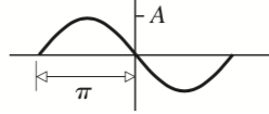
Figure 1. $\psi(x) = Asin(\frac{2\pi}{\lambda}x+\pi)$
2. A light wave (with phase velocity c = 3.00 × 10⁸ m s-1) has a wavelength of 1 μm.
Note that the visible region $\in \{400,...,700\}nm$.
(a) What frequency is the light?
$$c=\lambda \nu \implies \nu = \frac{c}{\lambda} = 3x10^{14}\space Hz$$(b) Is it in the visible range?
$$\frac{10^{9}\space nm }{1\space m}\frac{10^{-6} \space m}{} = 10^{3} nm$$$ \therefore$ this wavelength is just outside of the visible region.
3. An electron has a deBroglie wavelength of $1 Å$ = $1 × 10^{-10}\space m$.
(a) What is its momentum?
$$p = \frac{h}{\lambda} = 7x10^{-24} \space J.s.m^{-1}$$(b) Given the mass of the electron ($m_{e} = 9.109x10^{-31} \space kg$), what is the electron’s velocity?
Linear momentum is just:
$$ p = mv \implies v = \frac{p}{m} = 7x10^{6} m.s^{-1}$$4. Suppose we have confined an electron to a very small space, such that we can measure its position to an uncertainty of $∆x = 1 \space nm$. If we measure the momentum, what is the lower limit in the expected uncertainty $∆p$?
Heisenberg's Uncertainty Principle (1927):
$$\Delta x \Delta p \underline{>} \frac{\hbar}{2} \implies \Delta p \underline{>} \frac{\hbar}{2 \Delta x} = 5.27x10^{-26} J.s.m^{-1}$$5. Write down the 1D time-independent Schrodinger equation.
$$ \hat{H}\psi(x) = \overbrace{-\frac{\hbar^{2}}{2m}(\frac{\partial^{2} \psi(x)}{\partial x^{2}})}^{\text{Kinetic Energy}} + \overbrace{V(x)\psi(x)}^{\text{Potential Energy}} = E\psi(x)$$6. Write down normalized Particle-In-a-Box (PIB, i.e. $V(x) = 0$ inside a box of length $L$) wavefunctions $\psi_{n}(x)$ for $n=1, 2 \space and \space3$, and their corresponding energies $E_{n}$.
Just plug $n=1, 2 \space and \space3$ into the equations below...
$$\psi(x) = \sqrt{\frac{2}{L}}sin(\frac{n\pi x}{L}),$$where the eigenvalue of the Hamiltonian operator for PIB is just
$$E = \frac{h^{2}n^{2}}{8mL^{2}} $$7. Draw the PIB wavefunctions $\psi_{n}(x)$ for $n=1, 2 \space and \space3$.
8. Draw the probability distributions $P_{n}(x)$ for $n=1, 2 \space and \space3$.
Look at the image of PIB wavefunctions) for $n=1, 2 \space and \space3$ and reflect the negative portion of the curve into the positive region.
9. Suppose I give you an unnormalized wavefunction $\psi(x)$, and the information that $\int |\psi(x)|^{2}dx = 0.5$ . What number $c$ will produce a normalized wavefunction $c\psi(x)$ ?
$$\int c\psi(x)^{*}c\psi(x)dx = 1 \implies c^{2}\int |\psi(x)|^{2}dx = 1$$$$c^{2}\int |\psi(x)|^{2}dx = c^{2} \frac{1}{2} = 1$$$$c^{2} =2 \implies c = \sqrt{2}$$10. For PIB wavefunction $\psi_{n}(x)$, $n=2$, what is the probability that the electron will be found on the right most quarter of the box, i.e. $\frac{3L}{4} < x < L$? (Hint: draw a picture!)
Due to symmetry:
$$ P(x) = 0.25$$11. A diatomic $C=O$ molecule is excited from a $v=1$ vibrational state to a $v=2$ state by a light wave. (a) If the harmonic oscillator force constant is $1860 N. m^{-1}$, calculate the frequency of the light. (Hint: you will need to consider the reduced mass $\mu$).
The harmonic oscillator eneergy is just
$$ E_{v} = (v + \frac{1}{2})\hbar\omega,$$where
$$\omega = \sqrt{\frac{k_{f}}{\mu}},$$and
$$ \mu = \frac{m_{1}m_{2}}{m_{1}+m_{2}} = 1.147x10^{-26} \space kg $$The separation between adjacent energy levels is
$$E_{v+1}-E_{v} = \hbar \omega $$$$E_{2}-E_{1} = h \frac{1}{2\pi}\sqrt{\frac{k_{f}}{\mu}} $$$\therefore$
$$ \nu = 6.31x10^{13} \space Hz$$(b) Based on the frequency you compute, what kind of light is this (e.g. radio waves, UV, etc...)?
UV region
12. State how the energies En of the hydrogen-like wavefunctions depend on quantum numbers n, l and m?
$$E = -\frac{13.6 \space eV}{n^{2}} \implies E_{n} \propto -\frac{1}{n^{2}}$$$$E_{l,m_{l}} = l(l+1)\frac{\hbar^{2}}{2I} = \frac{|J|^{2}}{2I},$$where
$$ |J| = \sqrt{l(l+1)}\hbar$$13. The ground state of the hydrogen atom has an ionization energy of 13.6 eV. What is the ionization energy for the ground state of $He^{+}$?
$$ E_{n} = -\frac{Z^{2}(13.6 \space eV)}{n^{2}} = \frac{-4(13.6)}{1^{2}},$$where
$$I = -E \implies I = 54.4 \space eV$$14. What is the maximum number of electrons that can occupy n=3 states in an atom? (remember to count spin states too!)
Write out possible quantum numbers: $n = 3, \space l = \{0,1,2\}, \space m_{l}=\{-2,-1,0,1,2\}$
Max number of electrons in subshell is $2(2l+1)$, and the max number of electrons in a shell is $2n^{2}$.
Therefore,
$$\sum_{i=0}^{2} 2(2l_{i}+1) = 2(2(0)+1)+2(2(1)+1)+2(2(2)+1)= 18$$$$\text{or}$$ $$2(3)^2 = 18$$15. The ground-state radial wavefunction for the hydrogen-like atom (i.e. a $1s$ orbital) is $R(r) = 2(\frac{Z}{a_{0}})^{3/2} exp(-Zr/a_{0})$. What is the most probable radius r for the electron?
Then, we need to find the value of r that maximizes $P(r)$. Take first derivative and set equal to zero. Solve for r.
$$d P=\left[\frac{1}{\sqrt{\pi} a_{0}^{3 / 2}} e^{-r / a_{0}}\right]^{2} 4 \pi r^{2} d r=\frac{4}{a_{0}^{3}} r^{2} e^{-2 r / a_{0}} d r$$$$2 r e^{-2 r / a_{0}}-\frac{2}{a_{0}} r^{2} e^{-2 r / a_{0}}=0$$$$2 r e^{-2 r / a_{0}}[1 - \frac{r}{a_{0}}] = 0 \implies r = a_{0} = 0.529 Å$$Side Notes for 15.:
$$P(r) = \int_{0}^{\pi} \int_{0}^{2\pi} \int R^{2}|\Psi(\theta,\phi)|^{2} r^{2}sin(\theta)dr d\theta d\phi$$$$= \int r^{2} R^{2} dr \overbrace{ \int_{0}^{\pi} \int_{0}^{2\pi} \underbrace{|\Psi(\theta,\phi)|^{2}}_{\frac{1}{4\pi}}sin(\theta) d\theta d\phi}^{1},$$hence
$$\int_{0}^{\pi} \int_{0}^{2\pi} sin(\theta) d\theta d\phi = 4\pi$$Therefore, the general forms are:
$$P(r) = 4\pi r^{2} \psi^{2}$$and
$$ P(r) = r^{2}R(r)^{2}$$16. State the definition of angular momentum.
The total angular momentum is defined as
$$ |J| = \sqrt{l(l+1)}\hbar,$$where each component can be represented as
$$ |J| = \sqrt{J_{x}^{2}+J_{y}^{2}+J_{z}^{2}}$$17. State how angular momenta terms |J| and Jz are quantized for particle-on-a-ring (in terms of quantum numbers m and l.)
$$ |J| = \sqrt{l(l+1)}\hbar, $$Multiples of Plancks constant.
where $l\in \{0,1,2,...\}$, $J_{z} = {-\hbar, 0, \hbar}$ and $m_{l} = \{-1,0,1\}$.
18. What are the key differences between valence bond theory and M.O. theory?
Valance bond theory (VB) says electrons live in sparate valance orbitals $\psi_{a},\psi_{b}$. When they overlap a bond is formed. $\psi_{_{VB}} = \psi_{a}(1)\psi_{b}(2)\pm\psi_{a}(2)\psi_{b}(1)$ approximates by considering electrons in A.O valance shell.
Molecular orbital theory (M.O.) says that neuclei share electrons and $\psi$'s are spread over multiple nuclei. M.O. theory also constructs linear combinations of A.O.'s and is able to predict bond orders, orbital overlap, and make predictions about bond characteristics.
19. Draw a $\pi$ orbital as a sum of two p-orbitals $(2p_{z})_{a}$ and $(2p_{z})_{b}$, centered on nuclei $a$ and $b$, respectively. Write down a VB wavefunction for this arrangement.

Suggesting indistinguishable nature of the two electrons (ignoring spin):
$$\psi_{_{VB}} = (2p_{z})_{a} (1)\space (2p_{z})_{b}(2)\pm(2p_{z})_{a}(2)\space(2p_{z})_{b}(1),$$where electron 1 is found in $(2p_{z})_{a}$ and also found in $(2p_{z})_{b}$.
20. Discuss why the peptide bond is planar, in terns of the concepts of resonance and hybridization.
21. Which of the following multiple-electron wavefunctions are valid (i.e. are anti-symmetric)?
Use the inversion operator: $\psi(x_{1},x_{2}) = - \psi(x_{2},x_{1})$


a. $1s_{a}(1) + 1s_{b}(2)$
$\psi = 1s_{a}(2) + 1s_{b}(1)$
$\therefore$ symmetric
b. $1s_{a}(1)\space 1s_{b}(2) + 1s_{a}(2)\space 1s_{b}(1)$
$\psi = 1s_{a}(2) \space 1s_{b}(1) + 1s_{a}(1)\space 1s_{b}(2)$
$\therefore$ symmetric
c. $1s_{a}(1)\space 1s_{b}(2) - 1s_{a}(2)\space 1s_{b}(1)$
$\psi = 1s_{a}(2)\space 1s_{b}(1) - 1s_{a}(1)\space 1s_{b}(2) = -(1s_{a}(1)\space 1s_{b}(2) - 1s_{a}(2)\space 1s_{b}(1))$
$\therefore$ antisymmetric
22. Is the overlap integral $S$ for the orbitals shown below non-zero? Why or why not? Will these orbitals form a chemical bond? If so, will it be a $\sigma$ or a $\pi$ bond? What kind of symmetry will might have, $g$ or $u$?
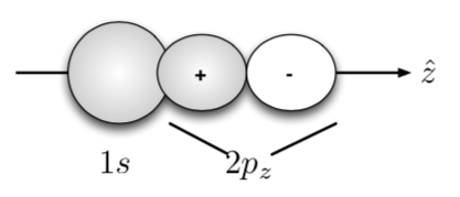

Why not? Consider $CH_{4}$!
Hint: Look at the shaded regions.
Answer:
Now, consider $1s_{a} + 2(p_{z})_{b} $. Writing as a linear combination for the bonding:
$$ \psi(1,2) = 1s_{a}(1)\space 2(p_{z})_{b}(2) + 1s_{a}(2)\space 2(p_{z})_{b}(1)$$Applying the inversion operator:
$$ \psi(2,1) = 1s_{a}(2)\space 2(p_{z})_{b}(1) + 1s_{a}(1)\space 2(p_{z})_{b}(2) = \psi(1,2)$$$\therefore$ symmetric $\rightarrow$ even.
$\sigma$-bond and $\sigma_{g}$
Jump to table of contents.
11.27 Consider the electrostatic model of the hydrogen bond. The $N–C$ distance of the hydrogen bonded groups in proteins, such as occur in an a helix, is $0.29 nm$. How much energy (in $kJ mol^{−1}$) is required to break the hydrogen bond
NOTE: partial charges (Units: $e^{-1}$) can be found in Table 11.2 —— Atkins.
(a) in a vacuum ($ε_{r} = 1$)
$$ E = -\frac{q_{C}q_{H}}{4\pi \epsilon_{0}\epsilon_{r}r_{CH}}+\frac{q_{C}q_{N}}{4\pi \epsilon_{0}\epsilon_{r}r_{CN}}+\frac{q_{O}q_{H}}{4\pi \epsilon_{0}\epsilon_{r}r_{OH}}+\frac{q_{O}q_{N}}{4\pi \epsilon_{0}\epsilon_{r}r_{ON}}$$Now, we take out $4\pi \epsilon_{0}\epsilon_{r}$ and pull out $e^{2}$ from the numerator.
$$ E = -\frac{e^{2}}{4\pi \epsilon_{0}\epsilon_{r}/e^{2}}(\frac{q_{C}q_{H}/e^{2}}{r_{CH}}+\frac{q_{C}q_{N}/e^{2}}{r_{CN}}+\frac{q_{O}q_{H}/e^{2}}{r_{OH}}+\frac{q_{O}q_{N}/e^{2}}{r_{ON}})$$$$ E = -\frac{e^{2}}{4\pi \epsilon_{0}\epsilon_{r}/e^{2}}(\frac{(0.45)(0.18)/e^{2}}{r_{CH}}+\frac{(0.45)(-0.36)/e^{2}}{r_{CN}}+\frac{(-0.38)(0.18)/e^{2}}{r_{OH}}+\frac{(-0.38)(-0.36)/e^{2}}{r_{ON}}) = 7.93x10^{-20} J$$$$ E =7.93x10^{-20} J *N_{A} = 47.8 kJ.mol^{-1}$$(b) in a membrane (essentially a liquid hydrocarbon with $ε_{r} = 2.0$)
Since $\epsilon_{r}$ increases by a factor of 2, then the energy should decrease by a factor of 2.
$$ E = 23.9 kJ.mol^{-1}$$(c) in water ($ε_{r} = 80.0$)?
Since $\epsilon_{r}$ increases by a factor of 80, then the energy should decrease by a factor of 80.
$$ E = 0.60 kJ.mol^{-1}$$11.44 We can explore bond torsion in ethane to understand the barrier to internal rotation of one bond relative to another in saturated carbon chains, such as those found in lipids. The potential energy of a $CH_{3}$ group in ethane as it is rotated around the $C–C$ bond can be written $V = \frac{1}{2} V_{0}(1 + cos(3\phi))$, where f is the azimuthal angle (24) and $V_{0} = 11.6 kJ mol^{−1}$.
(a) What is the change in potential energy between the trans and fully eclipsed conformations?
(b) Show that for small variations in angle, the torsional (twisting) motion around the $C–C$ bond can be expected to be that of a harmonic oscillator.
(c) Estimate the vibrational frequency of this torsional oscillation.
7.
Computer Lab – Spartan 4
Goal: The purpose of this lab is to illustrate how to use quantum chemical calculations to scan potential energy surfaces to determine molecular force field parameters. We will discuss two examples: (1) deriving the harmonic-oscillator force constant for a chemical bond, and (2) determining the preferred torsional minima for peptides.
Introduction
Last week we learned about calculating the energy of a protein as the sum of several pairwise energy terms (i.e. bonded terms, including bond distance, bond angle, and dihedral angle terms; and non-bonded terms, including electrostatics and van der Waals interactions). Such an energy function can be called a force field.
Here, we will work through two examples illustrating how QM calculations can be used to parameterize bonded interactions. First, we will scan the energy Eel(R) of an H2 molecule for different internuclear distance R. Then, we will scan peptide backbone dihedral angles to investigate preferred torsional minima for peptides.
Part 1: Potential energy surface for diatomic H2.
The energy of a bound diatomic molecule AB as a function of internuclear separation is described by its potential energy surface shown in Figure 1. The existence of a minimum of the potential energy surface (PES) implies there is a stable chemical bond between the two atoms. The minimum represents the equilibrium bond length Re of the molecule.
The energy of a bound diatomic molecule AB as a function of internuclear separation is described by its potential energy surface shown in Fig.1. The existence of a minimum of

Figure 1: Potential energy surface of a diatomic molecule A-B.
the potential energy surface (PES) implies there is a stable chemical bond between the two atoms. The minimum represents the equilibrium bond length Re of the molecule. A molecule however is not completely frozen but can vibrate around the minimum with some vibrational frequency νe. As the internuclear separation increases at values higher than minimum the energy increases also until the bond breaks and the two atoms are separated and they do not interact with each other any more. The energy at the dissociation limit is equal to the sum of the energies of the two atoms. The energy required to break the bond is the dissociation energy De. This potential can be described by a Morse potential
$$E^{el}(R) = D_{e}\{1 − exp [−\alpha(R − R_{e})]\}^{2} + C$$where $\alpha = \sqrt{\frac{k_{f}}{2D_{e}}}$. $k_{f}$ is the force constant defined as $k_{f} = (\frac{d^{2}E^{el}}{dR^{2}})_{R=R_{e}}$. The frequency of vibrational motion is given by:
$$\nu = \frac{1}{2\pi}\sqrt{\frac{k_{f}}{\mu}}$$The PES around the minimum can be approximated by a quadratic potential
$$E^{el}(R) = \frac{1}{2}k_{f}(R − R_{e})^{2} + c$$In this case the vibration of molecules is described by a Harmonic Oscillator.
Experimental procedure
Click here to use the Guest Server!
Step 1: As a first step in the study of the diatomic molecule $H_{2}$ you will obtain the equilibrium bond distance. Follow the WebMO instructions to build $H_{2}$ and optimize its structure at the CAS(2,2)/6-31G(d) level of theory. Choose optimization +frequency from the menu. After the calculation is finished report the optimized equilibrium geometry $R_{e}$ and the vibrational frequency $\nu_{e}$. At the minimum of the PES the first derivative of $E^{el}(R)$ with respect to $R$ is zero. The curvature is given by the second derivative $(\frac{d^{2}E^{el}}{dR^{2}})$ which at a true minimum is positive. The curvature is also related to the force constant and subsequently the vibrational frequency via Eq. 2. The above input will calculate the vibrational frequency after the optimization is finished (keyword: opt freq).
Step 2: a) Use WebMO to calculate the potential energy curve of $H_{2}$ at the CAS(2,2)/6- 31G(d) level. Choose bond lengths starting at 0.5 Å and increasing at an interval of 0.1 Å. (0.5, 0.6, 0.7, ...). The input is shown below:
#N CAS(2,2)/6-31G(d) Scan

H2

0 1
H
H 1 B1

B1 0.5 30 0.1
$$\overbrace{B1}^{\text{coordinate}} \underbrace{0.5}_{\text{bond length}} \overbrace{30}^{\text{# of calculations}} \underbrace{0.1}_{\text{interval}}$$
Using WebMO, build $H_{2}$ and choose a single point calculation at the CAS(2,2)/6- 31G(d) level at the job options window. Then go to the preview window and click on generate to generate the input. You will have to edit the input file so that it resembles the one above. Specifically you will have to change the SP keyword to SCAN. Then you will have to change the last line that gives the value of the coordinate B1. This should be (B1 0.5 30 0.1) as shown above. This line means that 30 single point calculations will be done where the bond length of $H_{2}$ will be varied. The first value will be 0.5 Å and then it will increase by 0.1 Å for 30 times. After you change the input submit the calculation. When the calculation is done, open the raw output file. Almost at the end of the file the summary of the calculation will be given. It will report:
Scan completed.


Summary of the potential surface scan: N B1 SCF
—- ——— ———–
1 0.5000 xxxxxx
and all the energies as a function of bond distance will be given. Plot the potential energy curve. Use the energy of the last point on the curve (which is close to the dissociation limit) to obtain the dissociation energy $D_{e}$.
Questions:
1. Report the equilibrium geometry Re in Å, vibrational frequency $\nu_{e}$ in wavenumbers, and dissociation energy De in eV.
2. Include a plot of the potential energy surface of $H_{2}$
Jump to table of contents.
%matplotlib inline
import plot as p
import numpy as np
x,y = np.loadtxt("scan551933.csv", skiprows=1, delimiter=",").transpose() # Energy is in Hartrees, where 1 Hartree = 27.2114 eV
y = y*27.2114 # eV
kf = 576. # N/m (tabulated value)
mp = 1.672*10**(-27.);m = 1.*mp
mu = m*m/(m+m) # kg
De, Re = (np.max(y)-np.min(y)), x[np.argwhere(y==np.min(y))][0,0]
nu = 1/(2*np.pi)*np.sqrt(kf/mu) # Get calculated kf by taking second derivative (R=Re)
p.simple_plot(x,y,xlabel='Coordinate ($\\AA$)',ylabel='Energy (eV)',Type='line',color=False,fig_size=(8,4),
              annotate_text=r'$R_{e} = %s Å$'%Re+"\n"+r'$D_{e} = %0.4G eV$'%De+"\n"+r'$\nu_{e} = %0.4G Hz$'%nu,
              annotate_x=2.0,annotate_y=-29)

Part 2: Potential energy surface for peptide backbone dihedral angles
Introduction
Last week we learned about calculating the energy of a protein as the sum of several pairwise energy terms (i.e. bonded terms, including bond distance, bond angle, and dihedral angle terms; and non-bonded terms, including electrostatics and van der Waals interactions). Such an energy function can be called a force field.
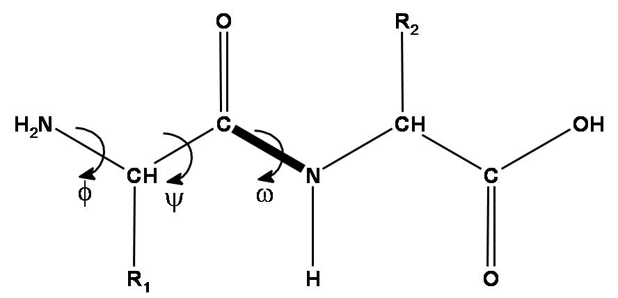
$$V(r)= \sum_{\text {bonds}} k_{b}\left(b-b_{0}\right)^{2}+\sum_{\text {angles }} k_{\theta}\left(\theta-\theta_{0}\right)^{2}+\sum_{\text {torsions }} k_{\phi}[\cos (n \phi+\delta)+1] \\ +\sum_{\text {nonbond }\\ \text{ pairs }}\left[\frac{q_{i} q_{j}}{r_{i j}}+\frac{A_{i j}}{r_{i j}^{12}}-\frac{C_{i j}}{r_{i j}^{6}}\right]$$The backbone dihedral angle (torsional) terms are of particular importance when developing force fields to describe the energetics of peptides. An incorrect torsional potential may bias protein conformations toward physically unrealistic conformations—i.e. too much alpha-helix or too much beta-sheet structure.
To get it right, all-atom force fields such as AMBER1 have been parameterized by adjusting the force constants to match quantum mechanical calculations of the total energy of a peptide molecule as a function of φ and ψ backbone dihedral angles. Our goal today is to perform a dihedral angle scan for the ψ angle of an amino acid residue (alanine, or any of your choice).
We will consider the following molecule:
Procedure
Build the molecule
Start building a new molecule using New Build. In the right-hand panel, choose the Peptide menu, and click on “Ala” (or another residue of your choice). Before adding it to your workspace, notice that you are given a choice of setting the dihedral angles (α, β, or Other). Click the “Other” button and set the custom dihedral angles to ψ = -180˚, φ= -60˚. Then click on the workspace to add the peptide.
Next, add capping groups to the peptide. Use the Organic menu on the right-hand side to cap the N-terminus with an acetyl group (C=O)CH3 and the C-terminus with an NH2 group.
Create copies of the molecule at different torsion angles
Go to Geometry > Set Torsions. Several yellow “cuffs” should show on each rotatable bond. For each dihedral angle except the ψ angle, click on the yellow cuff, and set Conformations to 0-fold = Off. Click on the ψ angle and set Conformations to 20-fold (9-fold).
Then, click the right-most button (with a black triangle pointing down) and generate a list of these conformers. If it goes well, you should be able to play an animation (left bottom) to see how it scans through.
Calculate the energy of each conformation
In Setup > Calculations… calculate “Energy” (not Equilibrium Geometry!) at the HF 6-31G* level in Vacuum (This is actually the basis set for the original AMBER parameterization (1994). Click Submit to submit the calculations.
It should take a minute or two – if you’d like you can monitor the job using Options > Local Monitor
Plot the results
After the calculation finishes, go to Display > Plots …
Click the green “+” to add a plot, with the molecule as the x-axis and E_kcal as the y-axis. Click the Merge button (little black triangle) to super impose the plot with the conformation. Cycle through to animation and see if you can identify the beta-sheet and alpha-helix minima.
Questions:
1. What intramolecular forces do you think are important in determining these minima?
Stabilization of peptide backbone (lowest energy) would take place at most favorable positions of lowest non-bonding interactions. Think about the peptide bond (between the carbonyl group of the first AA and amino group of the second AA) and its partial double bond character due to resonance. Varying $\psi$ the $C—C_{\alpha}$ bond clearly shows the non-bonded interactions that play a role between the carbonyl — $NH_{2}$ as well as the carbonyl — carbonyl upon rotation. Take note of the proximal changes for each of the rotations.
Note: The $\psi$ and $\phi$ angles are the 2 DOF that allow polypeptides to fold.
NOTE: This is the direction your scan should proceed:
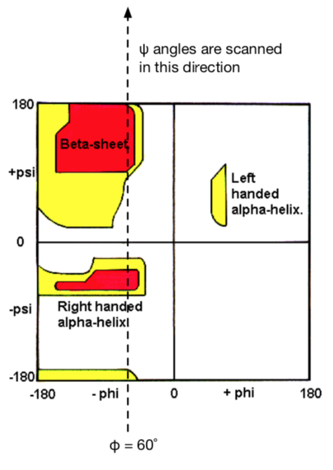
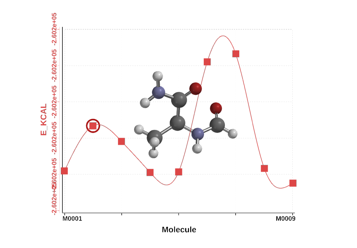
Figure 1. Dihedral scan about the $\psi$ angle of alanine with N-term capped with aldehyde and C-terminus capped with an NH2 group.
Cornell, W. D., Cieplak, P., Bayly, C. I., Gould, I. R., Merz, K. M., Ferguson, D. M., et al. (1995). A second generation force field for the simulation of proteins, nucleic acids, and organic molecules. Journal of the American Chemical Society, 117(19), 5179–5197. doi:10.1021/ja00124a002↩
Jump to table of contents.
8.
Computer Lab – Chimera 1
Goal: The purpose of this lab is to get familiar with protein structures determined by X-ray crystallography vs. nuclear magnetic resonance methods.
Introduction
In this exercise, we will use a protein called MDM2 as an example. MDM2 is an important protein in cancer—it has the ability to bind the transactivation domain of tumor suppressor protein p53, downregulating its ability to activate transcription. Many researchers have sought to develop anti-cancer drugs that target the binding site of MDM2, blocking p53 from binding, and thus upregulating the tumor suppressor activity of p53. Several of these drugs are currently in clinical trials.1
The first high-resolution atomic structure of MDM2 bound to p53 came from an X-ray crystal structure by Kussie et al. (1996).2 This structure shows a small helical region of p53 that binds a hydrophobic cleft in MDM2. To get these proteins to co-crystallize well, constructs with only residues 17-125 of MDM2, and residues 15-29 of p53, were used. Only the atomic structures of residues 25-109 could be resolved, however.
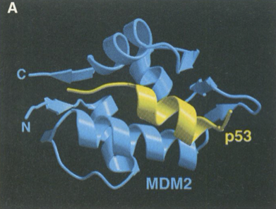
The X-ray crystal structure of MDM2-p53 (PDB ID: 1YCR)
In 2005, Uhrinova et al. used 2D NMR spectroscopy to determine the apo structure of MDM2 (“apo” = unbound by ligand).3 This structure contains more residues (1-119) but most of the terminal regions are unstructured.
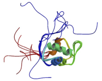
The NMR structure of apo-MDM2 (PDB ID: 1Z1M)
Viewing and visualizing PDB files
To find a given PDB structure, open a browser and go to http://pdb.org. In the search window, type in the PDB ID, which will bring you to the entry page. This page has a great deal of useful information about the protein sequence and structure.
To view the contents of the deposited PDB file containing the atomic coordinates, click on the Display Files drop-down in the upper right and choose PDB File. The full contents (text) of the PDB file should be viewable in your browser.
To view the molecular structure in 3D, open the Chimera application and choose File > Fetch by ID … Type the PDB ID into the text field and click Fetch. The ribbon structure of the protein should appear, which you can rotate in 3D by clicking and dragging.
Chimera Tips:
-
To view side chain atoms: Actions > Atoms/Bonds > show
-
A number of “preset” renderings are be found under the Presets menu
-
To select atoms, Control-click
-
To select multiple atoms Shift-Control click
-
Option-click and mouse drag to translate the view
-
If your view gets off-center for any reason, try Action > Focus to recenter.
Procedure
Use (1) the information in the Protein Data Bank (visual inspection of the *.pdb file, and molecular visualization in Chimera), and (2) the original publications (posted on Blackboard) to answer the questions below.
X-ray crystal structure of MDM2-p53
PDB: The atomic coordinates for this structure are deposited in the Protein Data Bank
under PDB ID: 1YCR.
Publication: Kussie, P. H., Gorina, S., Marechal, V., Elenbaas, B., Moreau, J., Levine, A. J., & Pavletich, N. P. (1996). Structure of the MDM2 oncoprotein bound to the p53 tumor suppressor transactivation domain. Science, 274(5289), 948–953.
Last week we learned about X-ray crystallography, and how it can be used to determine the atomic structure of proteins. Recall that this involves: (1) collecting diffraction data (i.e. the intensities of a large number of diffraction spots and their identification with Miller indices and a unit cell), and (2) using a model of protein electron density to calculate (by Fourier Transform) computed structure factors Fc that can be compared to the observed structure factors |Fo|.4
The resolution of the computed electron density depends on the number of diffraction spots (i.e. the number of “reflections”). To give you some sense of the resolution of the final model, consider Figure 1 from Kussie et al (1996) below:
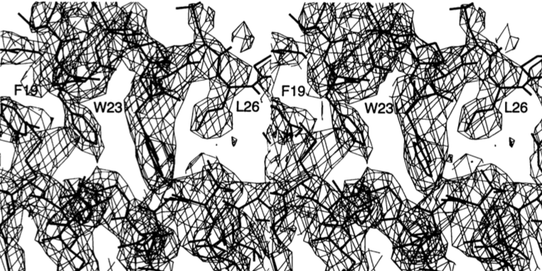
Figure. MIR electron density map of the X. laevis MDM2-p53 interface at 3.0 A resolution, contoured at 1.0 a, with the refined 2.3 A resolution atomic model in a stick representation. Stereo view focuses on the interactions of Phe19, Trp23, and Leu26 of p53 (labeled) with the (x2 helix of MDM2.
As you can see, the final model of the electron density really is “blobby”, but it is high-resolution enough that backbone and side-chain atoms (solid black lines, hard to see, I know) can be fit unambiguously. Some regions of this density may be too diffuse to fit (often the thermally mobile termini). For these regions, the protein structure is typically left undefined (hence, “missing residues” are common in X-ray crystal structures.)
-
Note that we are careful here to denote absolute values of Fo because of the so-called “phase problem” in which only intensities can be measured, not phase shifts.
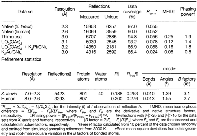
Table 1. Statistics from the crystallographic analysis.
Questions
-
Consider Table 1 from Kussie et al. (1996), in which statistics are given for a number of similar crystal structures the authors obtained.
-
Why is the number of unique reflections smaller than the total number?
-
Explain the correlation between the number of unique reflections and the resolution of the crystal structure.
The number of unique reflections represents a subset of the total measured reflections. The total number of measured reflections should contain measurements of equivalent symmetry elements.
The resolution increases with decreasing number of unique reflections.
-
-
The R-factor is a measure of the quality of the (electron density) model, defined as R = Σ|Fo - Fc|/ Σ|Fo|, where Fo and Fc are the observed and calculated structure factors, respectively. Because of the iterative refinement of computed structure factors from the observed data, there is a danger of overfitting. A more useful measure is called the Rfree value, where 10% of the observed structure factors are left out of the data set, so they can be used for testing the predictions.
-
Which should have the larger value, R or Rfree?
-
Based on the reported values for (human) MDM2-p53, do you think overfitting is a problem for this structure?
Rfree should
-
3. Why doesn’t this structure have any hydrogens?
Number of electrons are so small for hydrogen, such that the scattering factor is extremely low and will not be detected.
In Chimera, go to Tools > Higher-Order Structure > Unit Cell, and click Outline. Click on Make Copies to see the symmetrical copies of MDM2 inside the unit cell.
-
What are the unit cell dimensions a, b and c? (in Å, see also http://pdb.org)
-
What shape is the unit cell?
-
Visualize the side chains using wire-frame (Actions > Atoms/Bonds > Wire).
-
Based on what you can see, does it look like there are strong interactions between unit cell copies?
-
How careful do you think we need to be about such crystal packing artifacts when interpreting X-ray structures of proteins?
-
43.414, 100.546, 54.853
Rectangular prism
Recall that the crystallographic B-factor reports how diffuse the model of electronic density is for each atom. It is highly correlated to thermal motion. In Chimera, color the protein by B-factor, using Actions > Color > all options… > Tools > Render by Attribute (choose bfactor in the pull-down menu for Attribute:, then click Apply)
7. What parts of the protein have the most thermal motion?
NMR structure of apo-MDM2
PDB: The atomic coordinates for this structure are deposited in the Protein Data Bank
under PDB ID: 1Z1M.
Publication: Uhrinova, S., Uhrin, D., Powers, H., Watt, K., Zheleva, D., Fischer, P., et al. (2005). Structure of Free MDM2 N-terminal Domain Reveals Conformational Adjustments that Accompany p53-binding. Journal of Molecular Biology, 350 (3), 587– 598. doi:10.1016/j.jmb.2005.05.010
Solution structures of proteins are usually determined using 2D NMR spectroscopy. Two-dimensional techniques measure how the magnetization of one kind of nuclei (say, 1H) is affected by another kind of nuclei (say, 15N). The first step in 2D NMR is to assign the various magnetic resonances to particular protons. As long as the spectroscopic peaks are disperse (i.e. well-defined and far enough apart to be distinguished from one another), assignment is possible because resonance can only occur for nearby (through-bond) nuclei. For example, Figure 1 in
Uhrinova et al. (2005) shows HSQC (heteronuclear single quantum coherence) spectra disperse enough to assign (a) backbone NH protons and (b) side-chain protons.
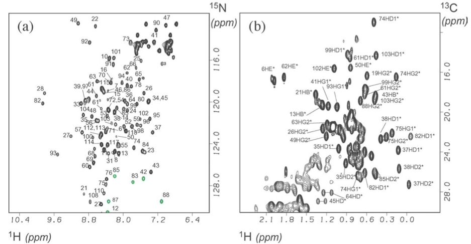
Figure. Assigned HSQC spectra of MDM2N. (a) 1H,15N HSQC spectrum. Folded peaks are shown in grey. HN–NH assignments are indicated by residue number. (b) A portion of the 1H,13C HSQC spectrum showing methyl groups, with assignments indicated by residue and atom identifier (based on CNS notation).
Once the peaks are assigned, studies of NMR relaxation times can determine the presence of Nuclear Overhauser Effects, or NOEs. An NOE is a short-range transfer of nuclear spin polarization from one nuclei to another that occurs through space (rather than through-bond). Like its optical cousin FRET (Förster Resonance Energy Transfer), it is an induced-dipole-dipole interaction that falls off as ~1/r6. If an NOE is observed between two protons, it means that they must be close in three-dimensional space, with the strength of the NOE related to proximity, for example:
-
Strong NOEs: 1.7 Å to 2.5 Å
-
Medium strong NOEs: 2.5 Å to 3.5 Å
-
Medium weak NOEs: 3.5 Å to 4.5 Å
-
Weak NOEs: 4.5 Å to 5.5 Å
A set of measured NOE distances can put enough restraints on the set of possible protein structures, so as to completely determine the solution conformation. A computer is used to explore possible structures that best satisfy the NOE distance restraints, generating an ensemble of different conformations, each equally compatible with the experimental restraints.
Questions
In Chimera, load structure 1Z1M.
-
Why does this structure include protons, whereas the X-ray crystal structure does not?
-
Why are there so many structures in this PDB?
-
Obviously, there are very few NOE distance restraints for the N-terminal region. The modeled ensemble has many possible conformations for this region. How well do you think this represents reality? In other words: how much is the conformational heterogeneity an artifact of the computer models used for structural refinement, versus a real feature of the MDM2 N-terminal region? Can you think of any other experimental biophysical methods that you could use to answer this question?
Bonus: Load both the X-ray structure (1YCR) and the NMR structure (1Z1M) into Chimera and align them using Tools > Structure Comparison > MatchMaker (select 1YCR as the reference, and shift-click to select all NMR structures to match).
4. Can you see any changes in the binding cleft as described by Uhrinova et al.?
Cornell, W. D., Cieplak, P., Bayly, C. I., Gould, I. R., Merz, K. M., Ferguson, D. M., et al. (1995). A second generation force field for the simulation of proteins, nucleic acids, and organic molecules. Journal of the American Chemical Society, 117(19), 5179–5197. doi:10.1021/ja00124a002↩
Hoe, K. K., Verma, C. S., & Lane, D. P. (2014). Drugging the p53 pathway: understanding the route to clinical efficacy. Nature Reviews Drug Discovery, 13(3), 217–236. doi:10.1038/nrd4236↩
Kussie, P. H., Gorina, S., Marechal, V., Elenbaas, B., Moreau, J., Levine, A. J., & Pavletich, N. P. (1996). Structure of the MDM2 oncoprotein bound to the p53 tumor suppressor transactivation domain. Science, 274(5289), 948–953.↩
Uhrinova, S., Uhrin, D., Powers, H., Watt, K., Zheleva, D., Fischer, P., et al. (2005). Structure of Free MDM2 N-terminal Domain Reveals Conformational Adjustments that Accompany p53-binding. Journal of Molecular Biology, 350(3), 587–598. doi:10.1016/j.jmb.2005.05.010↩
9.
Computer Lab – Chimera 2
Goal: The purpose of this lab is to get familiar analyzing protein-protein interfaces, and examine some of the energetic factors that contribute to favorable binding.
Introduction
Recall our friend from the last exercise, the MDM2-p53 complex (PDB ID: 1YCR).
The X-ray crystal structure of MDM2-p53 (PDB ID: 1YCR)
Let’s investigate how the p53 helix interacts with the MDM2 receptor.
Finding interacting residues
Load the structure using File > Fetch by ID … The ribbon structure of the protein complex should be shown
Select the p53 helix by Control-clicking (holding the CNTL key and clicking with the mouse) on p53, then press the up-arrow key to select the entire chain.
Find the receptor residues interacting with p53 using Tools > Surface/Binding Analysis.
In the “Atoms to Check” panel, click on the “Designate” buttons with the correct options so as to calculate interactions between the p53 helix (selected) and other atoms in the model.
In the “Clash/Contact Parameters” panel, click on “Contact” (not “Clash”). Then click on “Apply” below.
You should see a number of atoms in the helix and receptor selected. To select the residues involved, press the up-arrow key.
Visualize these residues using Actions > Atoms/Bonds > show. It may be helpful to Actions > Color > by element. (rendering as wire with a width of 4 works well too)
Questions
1. Which residues of p53 have the most interactions with the MDM2 receptor?
2. Which residues would you say are making hydrophobic interactions, and which have polar interactions?
Measuring surface area changes upon binding
Select the entire complex by control-clicking on any residue, and pressing the up-arrow key until the entire structure is selected.
Show the entire surface using Actions > Surface > show.
Calculate the total volume and surface area using Tools > Surface/Binding Analysis > Measure Volume and Area. The values are reported in units of Å3 and Å2, respectively. Write down these values in the table below.
Repeat these calculations for …
… the MDM2 receptor by itself (select the p53 helix and delete it using Actions > Atoms/Bonds > delete.), and
… the p53 helix by itself (reload 1YCR, select MDM2 only and delete it)
Chimera Commands:
We can obtain these calculations sing the command line interface:
Tools > General Controls > Command Line
We can generate a surface using the following command:
surface
You will need to generate separate surfaces for each chain. To select chain A:sel :.A; To select chain B:sel :.B; To select the surface sel #0:?
Once the surface is generated, measuing the surface area is easily obtained using the measure command:
measure area #0:?
measure volume #0:?
Chimera help page for buried surface area calculations
measure buriedArea :.A :.B
Chimera help page for buried surface area calculations
| 1YCR (entire complex) | MDM2 | p53 | |
|---|---|---|---|
| Volume (Å3) | $13.07x10^{3}$ | $11.11x10^{3}$ | 1531 |
| Surface Area (Å2) | 4556 | 4354 | 1092 |
Questions
1. What is the total change in surface area upon binding of the p53 helix to MDM2?
$$4354 + 1092 – 4556 = 890 Å^{2}$$2. Using the data from Figure 1a of Chen et al. (2013) below, make a rough estimate of the binding affinity of p53 helix (i.e. its dissociation constant Kd). Ask your TA for the actual answer
$$ {K_{d}}_{Exp} = 410 nM$$$${K_{d}}_{Approx} = 10^{log_{10} K_{d}} = 10^{-6}M = 1 uM = 1000 nM$$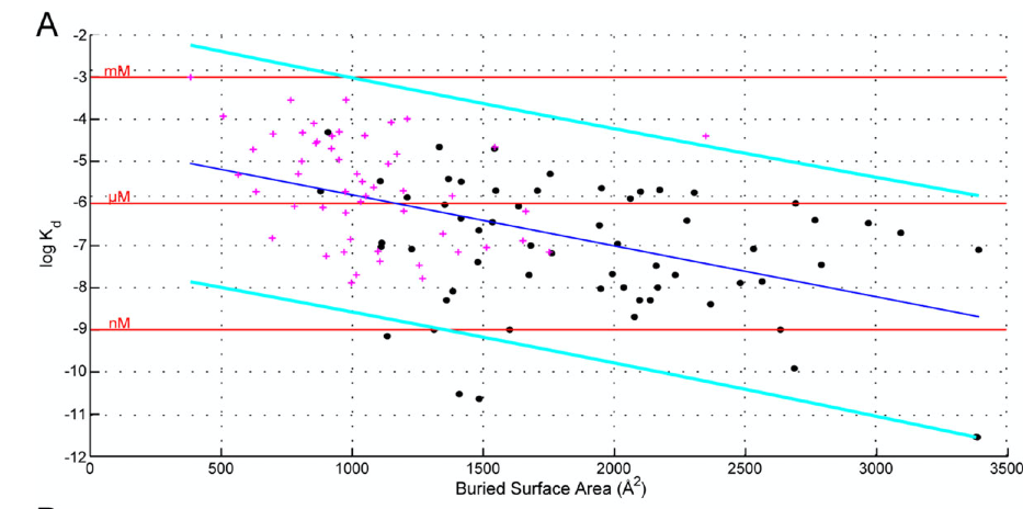
Figure 1a from Chen et al. (2013)1
Chen, J., Sawyer, N., & Regan, L. (2013). Protein-protein interactions: General trends in the relationship between binding affinity and interfacial buried surface area. Protein Science, 22(4), 510–515. doi:10.1002/pro.2230↩
Jump to table of contents.
10.
HW Review:
Chapter 11
11.1 What features in an X-ray diffraction pattern suggest a helical conformation for a biological macromolecule?
See Notes
11.2 Describe the phase problem in X-ray diffraction and explain how it may be overcome.
See Notes
11.12 It is observed that the critical micelle concentration of sodium dodecyl sulfate in aqueous solution decreases as the concentration of added sodium chloride increases. Explain this effect.

As $[\text{Sodium chloride}]$ $\uparrow$ the partial charge of the dodeyl sulfate heads are shielded by NaCl ions and as a result forms larger miscelles and $[\text{Sodium dodecyl sulfate}] \downarrow$.
Therefore,
$$[\text{Sodium dodecyl sulfate}] \downarrow as [\text{Sodium chloride}] \uparrow$$11.25 The glancing angle of a Bragg reflection from a set of crystal planes separated by 97.3 pm is 19.85°. Calculate the wavelength of the X-rays.
$$\lambda = 2dsin(\theta)$$Chapter 12
12.12 A swimmer enters a gloomier world (in one sense) on diving to greater depths. Given that the mean molar absorption coefficient of seawater in the visible region is 6.2 × 10⁻⁵ dm3 mol−1 cm−1, calculate the depth at which a diver will experience (a) half the surface intensity of light and (b) one-tenth that intensity.
Derivation of Beer's Law:
Here is an image of the situation we wish to model:
The density of particles, $\rho$ and the absorption coefficient, $\alpha$ multiplied by the intensity, I shown in the 1st order differential equation: $$ -\frac{\partial{I}}{\partial{x}} = I \alpha \rho $$
Combine like-terms to each side of the equation:
$$\int_{I_{0}}^{I} \frac{\partial{I}}{I} = -\int_{0}^{x} \alpha \rho \partial{x} $$We know that $\int \frac{1}{x}dx = ln(x)$, so
$$ln(\frac{I}{I_{0}}) = - \alpha \rho x, $$To get the general solution of the D.E we can take the exponential of both sides
$$\frac{I}{I_{0}} = e^{-\alpha \rho x} $$General Solution to the D.E:
$$I (x) = I_{0} e^{-\alpha \rho x}$$Otherwise, to continue deriving Beer's Law we can use the property of logarithms:
$$-ln(\frac{I}{I_{0}}) = ln(\frac{I_{0}}{I}) = \alpha \rho x, $$and since we know the following
$$log_{10}(x) = \frac{ln(x)}{ln(10)},$$then we can say
$$ log_{10}(\frac{I_{0}}{I}) = \frac{\alpha \rho x}{ln(10)}$$Finally, we can say that $\rho \propto c$. We can also simplify further by saying $\epsilon =\frac{\alpha}{ln(10)}$, which has units of $M^{-1}cm^{-1}$ and $x = b$, where b is in cm.
$$ A = ln(\frac{I_{0}}{I}) = \epsilon b c$$Now, solving for the path length $b$ gives the following expression with $c_{H_{2}O} = \rho/MW$ and $I = 0.5I_{0}$.
$$ b = \frac{ln(\frac{I_{0}}{0.5I_{0}})}{\epsilon (\rho/MW)} = \frac{0.301}{(6.2 x 10^{-5} dm^{3}. mol^{-1}.cm^{-1}) (55.5 mol.dm^{-3})} = 87 cm $$Note, since the information regarding salt water concentration is not provided in the question we approximated the concentration by with values for $H_{2}O$.
12.19 Assume that the electronic states of the p electrons of a conjugated molecule can be approximated by the wavefunctions of a particle in a one-dimensional box and that the dipole moment can be related to the displacement along this length by m = −ex. Show that the transition probability for the transition n = 1 $\rightarrow$ n = 2 is nonzero, whereas that for n = 1 $\rightarrow$ n = 3 is zero.
We can use parity to show that the transition probability for the transition n = 1 $\rightarrow$ n = 2 is nonzero.
Let $\psi_{n} = \sqrt{\frac{2}{L}}sin(\frac{n\pi x}{L})$, where
$$\mu_{fi} = < \psi_{f} | \vec{\mu} | \psi_{i} > $$Next, let (+) be an even function (does not change sign under inversion transformation) and (-) be an odd function such that:
$$(+)(-) = (-) \implies ≠ 0$$$$(+)(+) = (-)(-) = (+) \implies = 0$$For n = 1 $\rightarrow$ n = 2
$$\mu_{21} = <\psi_{2} | \vec{\mu} |\psi_{1} > \implies (-)(+) = (-) \implies <\psi_{2} | \vec{\mu} | \psi_{1} > \neq 0$$For n = 1 $\rightarrow$ n = 3
$$\mu_{31} = <\psi_{3} | \vec{\mu} |\psi_{1} > \implies (+)(+) = (+) \implies <\psi_{3} | \vec{\mu} | \psi_{1} > = 0 $$12.25 How many normal modes of vibration are there for (a) $NO_{2}$, (b) $N_{2}O$, (c) cyclohexane, and (d) hexane?
There are $3N-6$ and $3N-5$ vibrational modes (in which N is the number of atoms in molecule) for non-linear and linear molecules; respectively.
(a) $NO_{2}$, Non-linear; $3N-6 = 3(3)-6 = 3$
(b) $N_{2}O$, linear; $3N-5 = 3(3)-5 = 4$
(c) cyclohexane, non-linear; $3N-6 = 3(18)-6 = 48$
(d) hexane, non-linear; $3N-6 = 3(20)-6 = 54$
SIDE NOTES:
Rates of various processes
| $\text{Process}$ | $\text{Timescales (s)}$ | $\text{Radiative}$ | $\text{Transition}$ |
|---|---|---|---|
| IC | $10^{-14}-10^{-11}$ | N | $S_{n} \to S_{1}$ |
| Vib Relax | $10^{-14}-10^{-11}$ | N | ${S_{n}}^{*} \to S_{n}$ |
| Abs | $10^{-15}$ | Y | $S_{0} \to S_{n}$ |
| Fluor | $10^{-9}-10^{-7}$ | Y | $S_{1} \to S_{0}$ |
| ISC | $10^{-8}-10^{-3}$ | N | $S_{1} \to T_{1}$ |
| Phos | $10^{-4}-10^{0}$ | Y | $T_{1} \to S_{0}$ |
- timescale of FRET are typically in ns
12.37 When benzophenone is illuminated with ultraviolet radiation, it is excited into a singlet state. This singlet changes rapidly into a triplet, which phosphoresces. Triethylamine acts as a quencher for the triplet. In an experiment in methanol as solvent, the phosphorescence intensity Iphos varied with amine concentration as shown below. A time-resolved laser spectroscopy experiment had also shown that the half-life of the fluorescence in the absence of quencher is 29 ms. What is the value of $k_{Q}$?
| $Species$ | $\text{}$ | $\text{}$ | $\text{}$ |
|---|---|---|---|
| $[Q]/(mol\space dm^{−3})$ | 0.0010 | 0.0050 | 0.0100 |
| $I_{phos}/(A.U.)$ | 0.41 | 0.25 | 0.16 |
First, we need to write out the mechanism that is given in the question:
$$ M + h\nu_{i} \rightarrow M^{*} \tag{1}$$When benzophenone is illuminated with ultraviolet radiation, it is excited into a singlet state.
$$ M^{*} \rightarrow M + h\nu_{phos} \tag{2}$$This singlet changes rapidly into a triplet, which phosphoresces.
$$ M^{*} + Q \rightarrow M + Q \tag{3}$$Triethylamine acts as a quencher for the triplet.
To model this process, we apply the steady state approximation on $[M^{*}]$ to obtain $I_{phos}$... (Do this to get your own "stern-volmer" equation that models what the questions provides).
Steady State is an assumption that the rate of (production/destruction) is equal to zero i.e., at equilibrium.
$$\frac{d[M^{*}]}{dt} = I_{abs} - k_{Q}[Q][M^{*}]-k_{phos}[M^{*}]=0$$$$ \implies (-k_{Q}[Q]-k_{phos})[M^{*}] = -I_{abs} \implies [M^{*}] = \frac{I_{abs}}{k_{Q}[Q]+k_{phos}},$$and we know that $I_{phos} = k_{phos}[M^{*}]$, so
$$ I_{phos} = k_{phos} \frac{I_{abs}}{k_{Q}[Q]+k_{phos}}$$We can take the inverse of $I_{phos}$ to get the equation in the form of a line:
$$ \frac{1}{I_{phos}} = \frac{1}{I_{abs}} + \frac{k_{Q}[Q]}{k_{phos}I_{abs}}$$Now, we plot the data that was given and extract the slope...
%matplotlib inline
import plot as p
import numpy as np
Q = np.array([0.0010,0.0050, 0.0100])
Iphos = np.array([0.41, 0.25, 0.16])
x,y = Q,1/Iphos
p.simple_plot(x,y,xlabel=r'$[Q]$',ylabel=r'${I_{phos}}^{-1}$',Type='scatter',color=False,fig_size=(8,4),
              fit=True, order=1, annotate_text=r"$slope=k_{Q}/(k_{phos}I_{abs})$",annotate_x=-0.005, annotate_y=5.5)

Therefore, the linear fit gives: $$I_{phos}^{-1}=(424.5302 dm^{3} mol )[Q]+(1.966), $$
where $\frac{k_{Q}}{k_{phos}I_{abs}} = 424.5302 dm^{3} mol $.
Therefore,
$$k_{Q} = \frac{(24.5302 dm^{3} mol)(2.39x10^{4} s^{-1})}{1.97} = 5.2x10^{6} dm^{3} mol^{-1} s^{-1} $$Jump to table of contents.
12.39 The Förster theory of resonance energy transfer and the basis for the FRET technique can be tested by performing fluorescence measurements on a series of compounds in which an energy donor and an energy acceptor are covalently linked by a rigid molecular linker of variable and known length. L. Stryer and R.P. Haugland, Proc. Natl. Acad. Sci. USA 58, 719 (1967), collected the following data on a family of compounds with the general composition dansyl-(l-prolyl)n-naphthyl, in which the distance R between the naphthyl donor and the dansyl acceptor was varied by increasing the number of prolyl units in the linker:
| $\text{}$ | $\text{}$ | $\text{}$ | $\text{}$ | $\text{}$ | $\text{}$ | $\text{}$ | $\text{}$ | $\text{}$ | $\text{}$ | $\text{}$ |
|---|---|---|---|---|---|---|---|---|---|---|
| $R/nm$ | 1.2 | 1.5 | 1.8 | 2.8 | 3.1 | 3.4 | 3.7 | 4.0 | 4.3 | 4.6 |
| $\eta_{T}$ | 0.99 | 0.94 | 0.97 | 0.82 | 0.74 | 0.65 | 0.40 | 0.28 | 0.24 | 0.16 |
Are the data described adequately by the Förster theory (eqns 12.26 and 12.27)? If so, what is the value of $R_{0}$ for the naphthyl–dansyl pair?
Förster theory:
States that the efficiency of resonance energy transfer is related to the distance $R$ between donor-acceptor pairs by
$$\eta_{T} = \frac{{R_{0}}^{6}}{{R_{0}}^{6} + {R}^{6}}, $$where $R_{0}$ is the distance at which $50 \%$ of the energy is transfered from donor to acceptor, and $R$ is the distance between donor and acceptor.
First, we need to rearrange the Förster theory equation into a linearized form.
$$ \frac{1}{\eta_{T}} = \frac{{R_{0}}^{6} + {R}^{6}}{{R_{0}}^{6}} = 1 + (\frac{R}{R_{0}})^{6}$$Now, we are able to plot the data:
%matplotlib inline
import plot as p
import numpy as np
R = np.array([1.2, 1.5, 1.8, 2.8, 3.1, 3.4, 3.7, 4.0, 4.3, 4.6])
nT = np.array([0.99, 0.94, 0.97, 0.82, 0.74, 0.65, 0.40, 0.28, 0.24, 0.16])
x,y = R**6,1/nT
p.simple_plot(x,y,xlabel=r'$(R/(nm))^{6}$',ylabel=r'${\eta_{T}}^{-1}$',Type='scatter',color=False,fig_size=(8,4),fit=True, order=1)

1. Calculate the dipole moment of formamide (in units D), given the bond lengths and partial charges below:
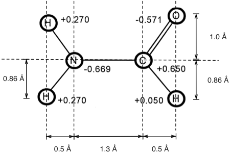 $$\mu = \sum_{i}q_{i}\vec{r}_{i},$$
where $r=\sqrt{x^{2} + y^{2}+z^{2}}$ and so each component is considered in the resultant dipole vector $\mu = \sqrt{{\mu_{x}}^{2} + {\mu_{y}}^{2}+{\mu_{z}}^{2}}$.
Here, in this problem we are given a molecule and coordinates in 2-D space, therefore we will only have two components.
$$\mu_{x} = \sum_{i}q_{i}x_{i} \hspace{0.5cm} \text{and} \hspace{0.5cm} \mu_{y} = \sum_{i}q_{i}y_{i} \tag{1}$$$$\mu = \sqrt{{\mu_{x}}^{2} + {\mu_{y}}^{2}} \tag{2}$$See Page 428 for more details.
import numpy as np
import pandas as pd
# Creating a dictionary for each of the atoms in the molecule
e = 1.602*10**(-19.) # C
atoms = {"H1":[0.270, (-1.3-0.5,0.86)], # [charge, (x,y)] in e and Å
        "O":[-0.571, (0.5,1.0)],
        "N":[-0.669, (-1.3,0.0)],
        "C":[0.650, (0.0,0.0)],         # deamed to be the origin
        "H2":[0.270, (-1.3-0.5,-0.86)],
        "H3":[0.050, (0.5,-0.86)]}
df = pd.DataFrame(atoms)
df
print("Atoms: %s"%[atom for atom in atoms.keys()])
print("Charges: %s"%[charge[0] for charge in atoms.values()])
print("Positions: %s"%[pos[1] for pos in atoms.values()])
mu_x = sum([atom[1][0]*e*atom[1][1][0]*10**-10. for atom in atoms.items()]) # see eq 1 above
mu_y = sum([atom[1][0]*e*atom[1][1][1]*10**-10. for atom in atoms.items()]) # see eq 1 above
print("mu_x,mu_y = %0.4g,%0.4g C m"%(mu_x,mu_y))
mu = np.sqrt(mu_x**2 + mu_y**2) # see eq 2 above
print("mu = %0.4g C m"%(mu))
mu = mu/(3.335*10**(-30.))
print("mu = %0.4g D"%(mu))
print("Experimental mu = %s"%(3.73) # Source given above
2. Two equal and opposite charges places 10 Å apart experience an attractive electrostatic force. Is this force stronger in water or in the gas phase? Why?
$$V(r) = \frac{q_{1}q_{2}}{4 \pi \epsilon_{r}\epsilon_{0} r^{2}}, $$where $q_{1}$ and $q_{2}$ are equal and opposite charges, the permittivity of free space $\epsilon_{0}$ = 8.854 × 10⁻¹² C2 J-1 m-1, $r=10 Å$ and the dielectric constant $\epsilon_{r}$ is different for both cases and depends on the medium. The dielectric constant is related to the effective electric field generated by interactions with the medium.
Therefore, the potential energy of the two charges separated by bulk water is reduced by nearly two orders of magnitude compared to the value it would have if the charges were separated by a vacuum. See Page 425 for more details.
3. True or False? The dielectric constant of water is 1.0.
False. The dielectric constant of water is 78. The dielectric constant of vacuum is 1.0
4. Are the dielectric properties of polar solvents due mainly to (a) atomic or (b) molecular polarization?
The larger the polarizability of the molecule, the greater is the distortion cause by a given strength of electric field. If the molecule contains large atoms with electrons some distance from the nucleus, the nuclear control is less and the polarizability of the molecule is greater. The polarizability also depends on the orientation of the molecule with respect to the field unless geometrically symmetric ($CH_{4}$, $SF_{6}$, etc.). See Pages 426-432 for more information.
5. Draw the Lennard-Jones potential, labeling the parts that are influenced by the r-12 term and the r-6 term.
Lennard-Jones Potential
$$V(r) = 4\epsilon[\overbrace{(\frac{\sigma}{r})^{12}}^{\text{Repulsion}} - \overbrace{(\frac{\sigma}{r})^{6}}^{\text{Attraction}}]$$At short ranges, the main contribution from the potential energy function comes from $(\frac{1}{r})^{12}$, which corresponds to the repulsive interactions (Pauli repulsion due to overlap of electron orbitals). At long ranges the main contribution from the potential energy function comes from $(\frac{1}{r})^{6}$,which corresponds to the attractive force (van der Waals force, or dispersion force).
Recall that the force is related to the potential energy by
$$F = - \frac{dV(r)}{dr} $$Find the distance $r$, at which the potential energy reaches a minimum.
Set the first derivative of the potential energy function equal to zero and solve for $r$.
Find $\sigma$, the distance $r$ at which the potential energy is zero.

See Page 436 for more details.
6. True or False: The polymer scaling law Rg ~ Nν for a protein in a compact globule state has an exponent ν = ½.
Jump to table of contents.
Spectroscopy
7. The molar absorption coefficient for a dye is ϵ = 12000 L/mol/cm for light of wavelength λ = 590 nm. At a dye concentration of 100 mM, what is the cuvette path length necessary to decrease the intensity of light by a factor of 10?
$$A = log(\frac{I_{0}}{I}) = -log(T) = \epsilon b c$$$$ b = -\frac{log(T)}{\epsilon c},$$where the intensity of light transmitted has decreased by a factor of 10, so $T=1-0.1 = 0.90$. Solve.
8. What is an isobestic point? What does observing an isobestic point say about the system you are studying?
The isobestic point is a specific wavelength at which the absorbance intensity of a sample is invariant during a chemical reaction and comes about when there are at least two interrelated absorbing species in solution.
This says that if an isobestic point is to occur, then the two species involved are related linearly by stoichiometry, such that the absorbance is invariant for one particular wavelength. See Page 469 for more details.
Also note that the isostillbic point is for fluorescence spectra.
9. What is a transition dipole moment? Given a ground-state wavefunction ψ0(x) and an excited-state ψ1(x), write down the formula for the dipole moment.
\begin{align} \mu_{fi} &= < \psi_{f} | \vec{\mu} | \psi_{i} > \\ \mu_{10} &= < \psi_{1} | \vec{\mu} | \psi_{0} > = \int \psi_{1}(x) \space \vec{\mu} \space \psi_{0}(x) dx, \end{align}where $\vec{\mu}$ is the electric dipole moment operator, and $ \psi_{i}$ and $ \psi_{f}$ are the wavefunctions for the initial and final states, respectively. See Page 469 for more details.
10. Is N2 vibrationally active? i.e. can its vibrational modes be studied by IR spectroscopy? Why or why not?
No. $N_{2}$ and $O_{2}$ are both infrared inactive since they do not possess vibrational modes that result in a change of dipole moment. See Pages 476-477 for more information.
11. How many vibrational modes are there for the linear molecule NO?
Linear molecule: $3N-5$
Non-Linear molecule: $3N-6$
12. UV light is used to optically excite a singlet S0 state to a S1 state, which decays to the triplet state T (which is “forbidden” from transition back to S0). What emission process does this describe? Over what range of time scales does this process occur?
Phosphorescent, seconds or fraction of seconds. For more information, see the table of Rates of various processes.
13. What kind of information can be obtained using FRET spectroscopy? What is the distance dependence of the FRET effect?
Förster resonance energy transfer (FRET) spectroscopy is useful for studying processes involving inter and intra-molecular energy transfer and can be used to measure distances (ranging from 1 to 9 nm) in biological systems. Furthermore, conformational changes can be studied, and also good for studying bulk distances. Single molecule FRET —create histograms of binned FRET distances, ultimately revealing states.See Pages 500,501 for more information.
Förster theory:
States that the efficiency of resonance energy transfer is related to the distance $R$ between donor-acceptor pairs by $$\eta_{T} = \frac{{R_{0}}^{6}}{{R_{0}}^{6} + {R}^{6}}, $$
where $R_{0}$ is the distance at which $50 \%$ of the energy is transfered from donor to acceptor (known value and varified by experiment), and $R$ is the distance between donor and acceptor. This dependence is related by
$$\eta_{T} \propto {R}^{-6} $$14. The fluorescence lifetime of tryptophan is τ0 = 2.6 ns. The ratio of fluorescence intensity with quencher (I) and without quencher (I0) was measured for a series of quencher concentrations [Q], as shown below. What is the quenching rate kQ for the quencher? Give correct units(!)
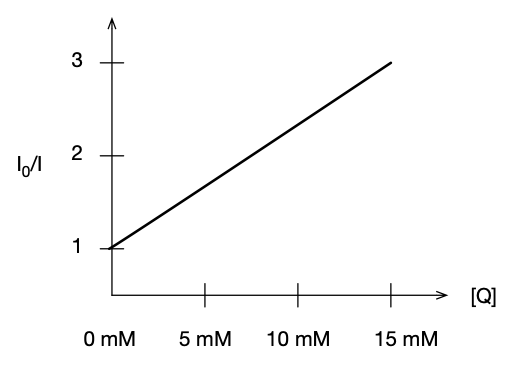
Because the fluorecence intensity and lifetime are both proportional to the fluorescence quantum yield, $I_{F,0}/I_{F}$ and $\tau_{0}/\tau$ against $[Q]$ should also be linear with the same slope and intercept. Therefore,
$$\frac{I_{F,0}}{I_{F}} = 1 + \tau_{0}k_{Q}[Q], $$where the slope = $\tau_{0}k_{Q}$. Now, we pick two points and get the slope of the line.
$$ slope = m = \frac{(y_{2} - y_{1})}{(x_{2} - x_{1})} = \frac{(3 - 1)}{(15 - 0)} = 0.13333 mM^{-1}$$$$k_{Q} = \frac{m}{\tau_{0}} = \frac{0.13333 mM^{-1}}{2.6 ns} = 0.0513 mM^{-1}ns^{-1}$$See Page 498 for more details.
Diffraction and crystallography
15. Draw two or more lines through the 2D lattice of points to show planes corresponding to Miller indices (2,1,0)
Did this in class...
$$(2,1,0) = (k,h,l)$$ $$2(\frac{1}{2},1,0) = (1,2,0)$$
16. The crystal unit cell of MDM2 has dimensions a = 43.4 Å, b = 100.5 Å, c = 54.8 Å. What is the spacing d of diffraction planes with Miller indices (2,1,0)?
\begin{equation} \frac{1}{d^{2}}=\frac{h^{2}}{a^{2}}+\frac{k^{2}}{b^{2}}+\frac{l^{2}}{c^{2}} \end{equation}See Page 418 for more information.
17. Describe the “phase problem” in X-ray crystallography, and at least one way the problem can be addressed (or at least circumvented to solve X-ray structures).
See Page 420 for phase problem, See Page 421 for the way the problem can be addressed.
Thermodynamics
18. What is the First Law of Thermodynamics?
Laws of Thermodynamics:
The 1st Law is concerned with the internal energy. We postulate that it obeys two properties. The first assumption made is that internal energy is extensive, which means it is additive.
$$ U = U_{1} + U_{2} $$The second assumption states that energy is conserved, states that energy can neither be created nor destroyed; energy can only be transfered or changed from one form to another e.g., $heat \rightarrow electrical$. Internal energy, $\Delta U$ of a system is the sum of the heat, $Q$ that flows across the system—surroundings barrier and the work, w done on the system by the surroundings:
$$ \Delta U = Q + w ,$$where work is defined as organized motion that can transfer energy.
where $Q > 0$ is when heat is absorbed by the system, and $Q < 0$ is when heat is transfered from system to surroundings. The previous equation can be summarized in the table below:
| Internal Energy, U | Heat, Q | Work, w | Physical Description |
|---|---|---|---|
| + | + | + | Heat flows into the system & Work done by the surroundings. |
| +/- | + | - | Heat flows into the system & Work done by the system. |
| +/- | - | + | Heat flows into the surroundings & Work done by the surroundings. |
| - | - | - | Heat flows into the surroundings & Work done by the system. |
Work
The work term has the general form, $dW = \int Fdx $ where $F$ is the applied force, and x is a mechanical extensive variable.
We already know that $P = F/A$, so lets substitute this in for F, and say that area, $A = x^{2}$. Then,
\begin{align} dW &= \int Fdx = \int P dx^{3}\\ dW &= \int_{V_{i}}^{V_{f}}P_{ext}dV = P(V_{f} - V_{i}) \end{align}where $V$ is the volume of a bulk system, and $p_{ext}$ is the external pressure.

In the diagram above, one can see that $w>0$ is related to compression and $w<0$ corresponds to expansion.
19. A volume of ideal gas is compressed at constant temperature. Does the internal energy $U$ increase?
Compression work
The question specifically says constant temperature (isothermal process) for an ideal gas. How can this increase $U$?
At constant temperature, the internal energy of the ideal gas should also be constant.
\begin{align} \Delta U &= Q + w\\ &= Q - P\Delta V,\\ \end{align}where $\Delta V = (V_{f} - V_{i}) < 0$ and $w>0$. Futhermore, the amount of heat released is the same as the work due to compression $Q = w$ $\therefore$ $\Delta U = 0$.
20. An ideal gas is slowly expanded from 1 L to 2 L at standard pressure and temperature.
(a) What is the work $w$ done on the system? (Make sure you have the correct sign!)
(b) What is the heat change $Q$ of the system?
Expansion work @ Constant P,T
$$-Q = w = -P\Delta V$$21. What is the mechanical work done for free expansion of a gas (say, in a vacuum)?
There is no work done when a system expands freely.
Since $P_{external} = 0$, then $w = -PdV = 0$
22. Consider the following reaction performed at a constant pressure of 1 bar, at 25˚ C = 298 K, with all species in the gas phase:
$$2 {NH_{3}}_{(g)} \rightarrow {N_{2}}_{(g)} + 3 {H_{2}}_{(g)}$$If we assume that all reactants and products behave like ideal gases, what is the expansion work done (in kJ/mol)? (Remember to carefully consider the sign of this value)
23. Draw a picture of the enthalpy H of water as a function of temperature T, from 75 ˚C to 125 ˚C (as it passes through the boiling point, Tb = 100 ˚C). Clearly label the heat of vaporization ∆Hvap.

Note that the temperature does not change during a phase change...
24. The heat capacity Cp of an unfolded protein is 8.0 kJ K-1 mol-1 at 350 K. Assuming Cp is relatively temperature-independent, calculate the change in enthalpy ∆H when the temperature is increased from 350 K to 375 K.
The following expression is derived in problem 25.
$$C_{P} = (\frac{\partial H}{\partial T})_{P} \implies dH = C_{P} dT$$$$ \Delta H = C_{P} \Delta T$$25. True or False? For an ideal gas, Cp + CV = nR
False.
By definition, heat capactiy is the ratio of the change in heat in an object to the change in temperature. The frist law of thermodynamics says:
\begin{align} dU &= \delta Q - \delta w\\ dU(\underbrace{S,V}_{\text{independent}\\\text{variables}}) &= TdS - PdV \end{align}Since $\delta Q = TdS$ and $\delta w = -PdV$, then
\begin{align} dU &= \delta Q - PdV\\ \text{At Constant V:} \hspace{1cm} (\frac{\partial U}{\partial T})_{V} &= (\frac{\partial Q}{\partial T})_{V} - P \underbrace{(\frac{\partial V}{\partial T})_{V}}_{\text{goes to 0}} = C_{V} \end{align}Use the equation of state for enthalpy to obtain $C_{P}$:
\begin{align} dH &= VdP + TdS\\ dH &= VdP + \delta Q\\ \text{At Constant P:} \hspace{1cm} (\frac{\partial H}{\partial T})_{P} &= V\underbrace{(\frac{\partial P}{\partial T})_{P}}_{\text{goes to 0}} + (\frac{\partial Q}{\partial T})_{P} = C_{P} \end{align}How do $C_{V}$ and $C_{P}$ relate to eachother?
$dQ = C_{V}dT+PdV$ $\hspace{0.5cm}$ and $\hspace{0.5cm}$ $dQ = C_{V}dT-VdP$
For an ideal gas: $PV = nRT$
\begin{align} C_{V}dT+PdV &= C_{P}dT - VdP\\ PdV + VdP &= C_{P}dT - C_{V}dT = (C_{P} - C_{V})dT\\ P(\frac{\partial V}{\partial T})_{P} V(\frac{\partial P}{\partial T})_{V} &= C_{P} - C_{V}\\ nR &\approx C_{P} - C_{V}, \hspace{0.25cm} \text{and} \hspace{0.25cm} C_{P} > C_{V} \end{align}13.
Computer Lab – SimBiology 1
Goal: The purpose of this lab is to become familiar with SimBiology by modeling a simple ligand binding reaction.
Introduction
Consider a binding reaction where ligand (L) binds to a protein receptor (R) to form a loosely bound encounter complex (L∙R), and finally a tightly bound product (P).1
$$L + R ⥂ L∙R \rightarrow P$$The SimBiology model of this receptor-ligand reaction looks like this (in MATLAB 2012a):
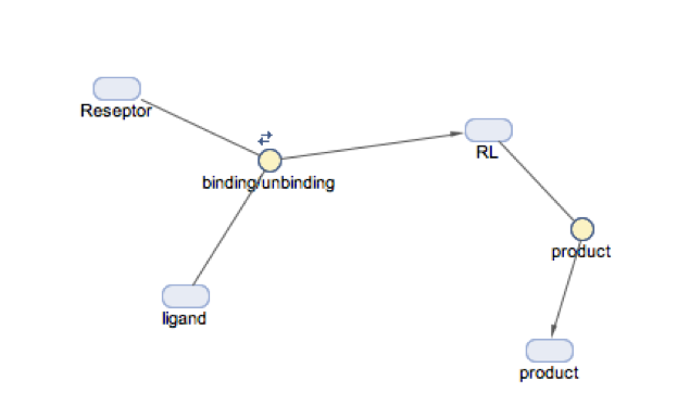
Let’s walk through the steps of how to build this model in SimBiology.
Procedure
Open Matlab and type simbiology at command window.
Go to Model tap in SimBiology window.
Home > add model > create new blank model
Model > Full > diagram
Rename window’s name to Receptor-Ligand reaction by double clicking on window.
Open Tools> Block Library Browser, Drag and drop three species and one reaction to the window.
Double click the name of the species and rename species to Ligand, Receptor and ligand-receptor respectively.
Rename reaction_1 to binding/unbinding
Hold down control key and draw an arrow from Ligand and Receptor to binding/unbinding
Draw an arrow from binding/unbinding to ligand-receptor
Double click on Ligand and set initial amount to 10.0
Double click on Receptor and set initial amount to 5.0
Double click on binding/unbinding
and check “reversible”
select “MassAction” for KineticLaw
set “Forward Rate Parameter” value to 0.02
set “Reverse Rate Parameter” value to 0.01
Run the simulation and save the graph.
Add another “species” and “reaction”. Name the species product and reaction as k-prod.
Connect ligand-receptor to k-prod and k-prod to product.
Select MassAction for kinetic law of k-prod and set value to 0.05.
Run simulation.
Does the reaction reach a steady state?
If not, increase simulation time to 100 by going to “simulation setting” (ask your TA if you can’t find it)
Repeat simulation for following values:
“Forward Rate Parameter” : 0.01 , “Reverse Rate Parameter” : 0.02 , “k-prod” : 0.05
“Forward Rate Parameter” : 0.02, “Reverse Rate Parameter” : 0.01 , “k-prod” : 0.5
Bonus
This same reaction can be used to describe Michaelis-Menten enzyme kinetics, in which substrate (S) binds a protein enzyme (E) to form an encounter complex (E∙S), and then chemically converts to product (E + P).
$$E + S \underset{k_{-1}}{\stackrel{k_{1}}{⥂}} E∙S \stackrel{k_{cat}}{\to} E + P$$Suppose an enzyme has k1 = 107 s-1, k-1 = 106 s-1 and kcat = 104 s-1. By adjusting parameters in SimBiology, which of these rates constants would you say most sensitively controls the overall rate of catalysis?
Note that this last kinetic step is “one-way”, which violates thermodynamics (!). Don’t worry about this yet (we’re getting to kinetics soon in the lecture). For now, suffice it to say that here we invoke the assumption that the back rate is very small compared to forward rate.↩
14.
Computer Lab – SimBiology 2
Goal: The purpose of this lab is to compare two- and three-state models of protein folding kinetics using the steady-state approximation
Introduction
This exercise is based on the following paper:
Teilum, K., Maki, K., Kragelund, B. B., Poulsen, F. M., & Roder, H. (2002). Early kinetic intermediate in the folding of acyl-CoA binding protein detected by fluorescence labeling and ultrarapid mixing. Proceedings of the National Academy of Sciences of the United States of America, 99(15), 9807–9812. doi:10.1073/pnas.152321499
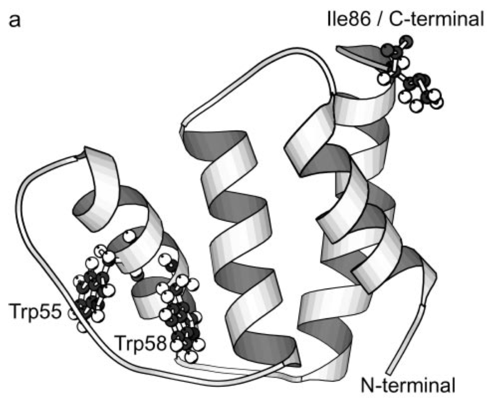
In this work, the folding kinetics of an 86-residue four helix-bundle protein called ACBP (acyl-CoA binding protein) was measured using time-resolved fluorescence spectroscopy (monitoring UV tryptophan fluorescence at 280 nm), after fast dilution from chemical denaturant (guanidinium hydrochloride, GuHCl) in a capillary mixer. The authors find that their data can be fit to the following kinetic model,
$$ U \underset{k_{IU}}{\stackrel{k_{UI}}{\rightleftharpoons}} I \underset{k_{NI}}{\stackrel{k_{IN}}{\rightleftharpoons}} N $$where U is a highly fluorescent unfolded state, I is a partially folded intermediate, and N is the folded state.
Procedure
Modeling the three-state mechanism
Use SimBiology to construct a model of the three-state folding kinetics, using the following kinetic rate parameters determined by the authors at 299 K:
$$ U \underset{k_{IU}= 7000 s^{-1}}{\stackrel{k_{UI} = 11000 s^{-1}}{\rightleftharpoons}} I \underset{k_{NI} = 0.07 s^{-1}}{\stackrel{k_{IN} = 650 s^{-1}}{\rightleftharpoons}} N $$Here is some experimental data that might be helpful in validating your model
| Time (ms) | Fluorescence intensity for the U state High concentration = more intensity |
|---|---|
| 0.2 | 1.1 |
| 0.4 | 1.0 |
| 0.6 | 0.98 |
| 0.8 | 0.96 |
| 1 | 0.91 |
| 2 | 0.6 |
| 20 | 0.33 |
| 40 | 0.32 |
| 60 | 0.31 |
| 80 | 0.29 |
Using initial concentrations of [U] = 10.0, [I] = 0.0, and [N] = 10.0, visualize the concentrations of each species over time. Draw or print/plot the results below.
Using the results of your SimBiology model, estimate the populations of U and N at equilibrium.
Estimate from this the equilibrium constant K = [Nequilibrium]/[Uequilibrium] and the free energy of folding.
Modeling the two-state mechanism
Let’s now apply the steady-state approximation to this three-state model. This approximation is a simplification saying that the concentration of the intermediate [I] is constant throughout the reaction. Since the formation of the intermediate is fast compared to the slower, rate-limiting step of folding to the native state N, the steady-state approximation is still fairly accurate.
To find the steady-state approximation, we go through the following steps:
1. Write down an expression for d[I]/dt :
$$\frac{d[I]}{dt} = -k_{IU}[I] - k_{IN}[I] + k_{UI}[U] + k_{NI}[I]$$2. Solve $\frac{d[I]}{dt} = 0$ (i.e. steady-state conditions) to get $[I]$ as a function of $[U]$ and $[N]$ :
\begin{align} 0 &= -k_{IU}[I] - k_{IN}[I] + k_{UI}[U] + k_{NI}[N]\\ [I](k_{IU} + k_{IN}) &= k_{UI}[U] + k_{NI}[N]\\ [I] &= (k_{UI}[U] + k_{NI}[N])/(k_{IU} + k_{IN}) \end{align}3. Next, we plug this expression for $[I]$ into the rate laws for $[U]$ and $[N]$:
\begin{align} \frac{d[U]}{dt} &= -k_{UI}[U] + k_{IU}[I]\\ &= -k_{UI}[U] + k_{IU} (k_{UI}[U] + k_{NI}[N])/(k_{IU} + k_{IN})\\ \frac{d[N]}{dt} &= -k_{NI}[N] + k_{IN}[I]\\ &= -k_{NI}[N] + k_{IN} (k_{UI}[U] + k_{NI}[N])/(k_{IU} + k_{IN}) \end{align}4. Finally, to get rates for a two-state $U\rightleftharpoons N$ model of folding, consider that at equilibrium, $\frac{d[U]}{dt} = \frac{d[N]}{dt} = 0$. Set the two expressions for $\frac{d[U]}{dt}$ and $\frac{d[N]}{dt}$ above to be equal to each other, and rearrange the equation to get it in the following form:
$$k_{forward} [U] = k_{backward}[N]$$What are your computed values of for $k_{forward}$ and $k_{backward}$? (Hint: They should be close to the values of $k_{IN}$ and $k_{NI}$, since $I \to N$ is the rate-limiting step.)
Estimate from $k_{forward}$ and $k_{backward}$ the equilibrium constant ($K = k_{f}/k_{b}$) and free energy of folding.