Validity of Molecular Simulations: Sampling Quality and Quantification of Uncertainty
Voelz Lab Group Meeting: October 2nd, 2019
by Robert M. Raddi
Motivation:
Massive amounts of care is involved with setting up the simulations. How much time is spent thinking about the validity?
Why should we care about statistical uncertainties?
- it's essential in molecular simulation
- we need to know how much we can trust our simulations
- Systems are getting larger and more complex
- No single method has emerged as a clear best practice to quantifying uncertainty (QU)
Grossfield, Alan, et al. "Best Practices for Quantification of Uncertainty and Sampling Quality in Molecular simulations [Article v1. 0]." Living journal of computational molecular science 1.1 (2018).
Convergence in the context of simulations:
- the extent to which an estimator approaches the "true value" (i.e., expectation of some observable) with increasing amounts of data.
- lack of convergence indicates sampling is poor
Hard part: it's highly likely that we don't know the "true value"
Configuration distance as a measure of convergence
How can we tell is sampling is good or bad?
Good:
- if there exists numerous transitions among apparent metastable regions $\implies$ adequate sampling for the configuration space
Bad:
- if the time trace exhibits only a few transitions
Concerns:
- degeneracy issue $\rightarrow$ many different configurations could have the same distance metric
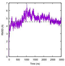
Figure 1. RMSD as a measure of convergence. $\alpha$-carbon RMSD of the protein rhodopsin from its starting structure as a function of time.
Grossfield, Alan, et al. "Best Practices for Quantification of Uncertainty and Sampling Quality in Molecular simulations [Article v1. 0]." Living journal of computational molecular science 1.1 (2018).
Configuration distance as a measure of convergence
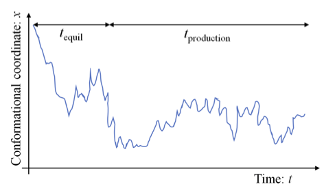
Figure 2. The equilibration and production segments of a trajectory. “Equilibration” over the time $t_{equil}$ represents transient behavior while the initial configuration relaxes toward configurations more representative of the equilibrium ensemble.
- sensitivity of $t_{production} \implies $ additional sampling is required
Grossfield, Alan, et al. "Best Practices for Quantification of Uncertainty and Sampling Quality in Molecular simulations [Article v1. 0]." Living journal of computational molecular science 1.1 (2018).
Autocorrelation analysis to estimate the standard uncertainty:
We wish to compute the number of independent samples in a time series, then find the standard uncertainty
this is performed by computing the autocorrelation function $g(\tau)$ for a set of lags $j$
Independent samples in a time series:
$$N_{ind} = \frac{N}{1+2\sum_{j=1}^{N_{max}} g(\tau)_{j}},$$where $N_{max}$ is the maximum number of lags.
Autocorrelation function:
$$ g(\tau) = \frac{<(x(t)-\bar{x})(x(t+\tau)-\bar{x})>}{\underbrace{s(x)^{2}}_{Variance}} $$Standard Uncertainty:
$$s(\bar{x}) = \frac{s(x)}{\sqrt{N_{ind}}} $$Correlation time ($\tau_{c}$):
Autocorrelation curve
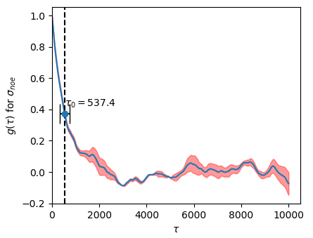
Figure 3. Autocorrelation curve for a MCMC simulation of Cineromycin (NOE) with 100k steps.
- correlations between a single observable at different times depend only on the relative spacing $\tau$ ("lag") between time steps.
- compute $g(\tau)$ for a set of lags $\tau$ i.e., two sliding windows (subtracted mean) moving against eachother while taking their dot product at each tau, $<(x(t)-\bar{x})(x(t+\tau)-\bar{x})>$
Sometimes we need get a better picture/understanding of the time-series...
Configuration distance as a measure of convergence
Block Averaging:
- a projection of a time series onto a smaller dataset of (approx.) independent samples so there is no need to compute the number of independent samples $N_{ind}$
$N$ observations ${x_{1},...,x_{N}}$ are converted to a set of M "block averages" ${{x_{1}}^{b},...,{x_{M}}^{b}}$, where
$${x_{j}}^{b} = \frac{\sum{k=1+(j-1)n}^{jn} x_{k}}{n} $$From here, we compute the arithmetic mean of the block averages $\bar{x}^{b}$. Followed by computing the standard deviation of the block averages $s(\bar{x}^{b})$.
Standard uncertainty of $\bar{x}^{b}$:
$$ s(\bar{x}^{b}) = \frac{s(x^{b}}{\sqrt{M}},$$which is used to calculate the confidence interval on $\bar{x}^{b}$.
- partition between continuous blocks and compute $g(\tau)$ for a collection of lags $\tau$, and average blocks to produce new $g(\tau)$
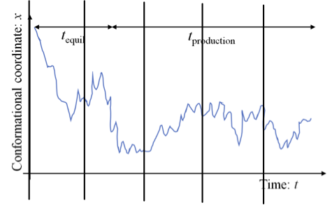
Figure 4. Partitioned trajectory partitioned into 5 continuous blocks.
Grossfield, Alan, et al. "Best Practices for Quantification of Uncertainty and Sampling Quality in Molecular simulations [Article v1. 0]." Living journal of computational molecular science 1.1 (2018).
Varying the starting positons of the sampling chain:
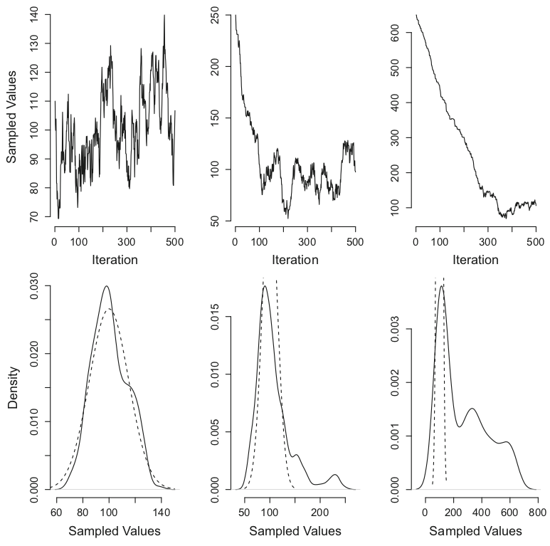
Figure 5. A simple example of MCMC. Left column: A sampling chain starting from a good starting value, the mode of the true distribution. Middle column: A sampling chain starting from a starting value in the tails of the true distribution. Right column: A sampling chain starting from a value far from the true distribution. Top row: Markov chain. Bottom row: sample den- sity. The analytical (true) distribution is indicated by the dashed line Van Ravenzwaaij, Don, Pete Cassey, and Scott D. Brown. "A simple introduction to Markov Chain Monte–Carlo sampling." Psychonomic bulletin & review 25.1 (2018): 143-154.
Bootstrapping:
Assuming data is uncorrelated...
Other Techniques of Bootstrapping and Block Averaging:
If the data is correlated — two options:
block covariance analysis (BCOM)
Hess, Berk. "Convergence of sampling in protein simulations." Physical Review E 65.3 (2002): 031910.
Assessing Uncertainty in Enhanced Sampling Simulations:
Replica Exchange Molecular Dynamics (REMD)
$^{*}$ Grossfield, Alan, et al. "Best Practices for Quantification of Uncertainty and Sampling Quality in Molecular simulations [Article v1. 0]." Living journal of computational molecular science 1.1 (2018).