Steps Towards Modeling Active Particles
Reviewing: Reentrant phase behavior in active colloids with attraction
May 6th, 2019
by Robert M. Raddi
$\renewcommand{\hat}[1]{\widehat{#1}}$
Outline
I. Discuss the main Ideas from Reentrant phase behavior in active colloids with attraction
II. Steps
- Create a basic 2-D LJ liquid simulation using velocity-Verlet algorithm and compare with Lammps
III. Prospective steps:
- Modify the 2-D LJ liquid simulation to match the paper.
- Does this model give us the full story?
IV. Conclusion
Motivation
Active particles
- Study active particles a new hot topic in liquids.
- Active fluids generally contain self-propelled particles that interact, individually endergonic, but as a collection generate large scale motion. [1]
At Low Reynolds Number: Self-propulsion (examples)
- Self-propelled colloids, bacteria, cells, algae and other micro-organisms.
Is it possible to uncover the dynamics of activity and interparticle attraction?
Reentrant phase behavior in active colloids with attraction
Redner, Gabriel S., Aparna Baskaran, and Michael F. Hagan. "Reentrant phase behavior in active colloids with attraction." Physical Review E 88.1 (2013): 012305.
DOI: 10.1103/PhysRevE.88.012305; Supplemental Information
$$ U = \frac{\epsilon}{k_{B}T} \hspace{0.5cm};\hspace{0.5cm} P_{e} = v_{P} \frac{\tau}{\sigma} $$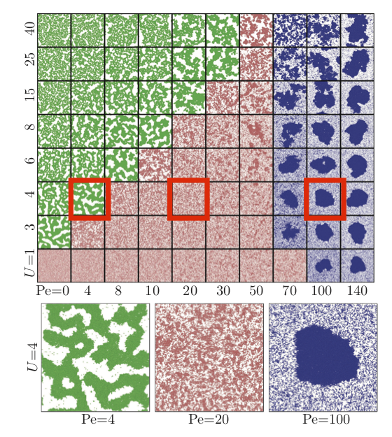
Stochastic Orientation of particles due to $\hat{\boldsymbol{v}}_{i} = (cos\theta_{i},sin\theta_{i})$
• High density phase $\rightarrow$ Low density phase: Modeled by an escape cone on the interface
Redner, Gabriel S., Aparna Baskaran, and Michael F. Hagan. "Reentrant phase behavior in active colloids with attraction." Physical Review E 88.1 (2013): 012305.
Interparticle attraction strength, U = 4
Propulsion Strength, $P_{e}$ = 4
Attractive interactions dominate and phase separation between gel and gas phase. As $t \rightarrow \infty$, gel $\rightarrow$ single cluster.
Redner, Gabriel S., Aparna Baskaran, and Michael F. Hagan. "Reentrant phase behavior in active colloids with attraction." Physical Review E 88.1 (2013): 012305.
Interparticle attraction strength, U = 4
Propulsion Strength, $P_{e}$ = 20
Activity is increased, which results in a single-phase (homogenous liquid).
Redner, Gabriel S., Aparna Baskaran, and Michael F. Hagan. "Reentrant phase behavior in active colloids with attraction." Physical Review E 88.1 (2013): 012305.
Interparticle attraction strength, U = 4
Propulsion Strength, $P_{e}$ = 100
Activity is increased further, which results in self-trapping that drives the system to phase separate again. Many initial clusters $\rightarrow$ single cluster.
Redner, Gabriel S., Aparna Baskaran, and Michael F. Hagan. "Reentrant phase behavior in active colloids with attraction." Physical Review E 88.1 (2013): 012305.
Brownian Motion
Coupled Overdamped Langevin Equations
Note that the equations of motion are nondimensionalized using time as $\tau = \sigma^{2}/D$, where $\sigma$ and $k_{B}T$ as basic units of length and energy.
$$\dot{r}_{i}=\text { Force }+\text { propulsion velocity w/ stochastic orientation}+\text { stochastic viscosity (Gaussian white noise) }$$$$\dot{\boldsymbol{r}}_{i}=\frac{1}{\gamma} \boldsymbol{F}_{\mathrm{LJ}}\left(\left\{\boldsymbol{r}_{i}\right\}\right)+v_{\mathrm{p}} \hat{\boldsymbol{v}}_{i}+\sqrt{2 D} \boldsymbol{\eta}_{i}^{\mathrm{T}},\label{eq:1}\tag{1}$$where $\eta$ is Gaussian white noise with $\left\langle\eta_{i}(t)\right\rangle= 0$ and $\left\langle\eta_{i}(t)\eta_{j}\left(t^{\prime}\right)\right\rangle=\delta_{i j} \delta\left(t-t^{\prime}\right)$. The magnitude of self-propulsion velocity is $v_{\mathrm{p}}$ and the direction of propulsion depends on the particles orientation, $\hat{v}_{i}=\left(\cos \theta_{i}, \sin \theta_{i}\right)$.
The angles associated with $\hat{v}_{i}$ are given by
$$\hat{\theta}=\sqrt{2 \mathcal{D}_{r}} \eta_{i}^{R},$$where the the rotational diffusion constant, $D_{r}$ goes to $D_{r} = 3D/\sigma^{2}$ at a low Reynolds number.
Lastly, the last term in equation $\ref{eq:1}$ directly relates to the stokes drag coefficient:
$$D=\frac{k_{\mathrm{B}} T}{\gamma}$$Table 1. Reduced Lennard-Jones Units:
| Quantity | Symbol | Relation to SI | Type |
|---|---|---|---|
| Mass | $m*$ | $m* = m M^{-1}$ | float |
| Positions | $r*$ | $x*=x\sigma^{-1}$ | np.array |
| Velocities | $v*$ | $$v* = v M^{1/2}\sigma^{-1/2}$$ | np.array |
| Energy | $E*$ | $E* = E \epsilon^{-1}$ | float |
| Temperature | $T*$ | $T* = T k_{B}\epsilon^{-1}$ | float |
| Forces | $F*$ | $F* = F \sigma \epsilon^{-1}$ | np.array |
| time | $t*$ | $t* = t\sigma^{-1} (\epsilon M^{-1})^1/2$ | float |
| Pressure | $P*$ | $P* = P \sigma^{dim=2} \epsilon^{-1}$ | float |
| Density | $\rho*$ | $\rho* = \rho \sigma^{dim=2}$ | float |
| Dynamic viscosity | $\eta*$ | $\eta* = N \sigma^{3} V^{-1}$ | float |
2-D Molecular Dynamics Simulation w/ LJ Potential
1. Initialize positions & velocities, setting t=0.
$$r_{x,y} = \left( \begin{array}{c}{r_{x1} \hspace{0.25cm} r_{y1}} \\ {r_{x2} \hspace{0.25cm} r_{y2}} \\ { \vdots}\hspace{0.25cm}{ \vdots} \\ {r_{\mathrm{xN}} \hspace{0.25cm} r_{\mathrm{yN}}}\end{array}\right) \hspace{0.35cm};\hspace{0.35cm} v_{x,y} = \left( \begin{array}{c}{v_{x1} \hspace{0.25cm} v_{y1}} \\ {v_{x2} \hspace{0.25cm} v_{y2}} \\ { \vdots}\hspace{0.25cm}{ \vdots} \\ {v_{\mathrm{xN}} \hspace{0.25cm} v_{\mathrm{yN}}}\end{array}\right) $$Determine the kinetic energy
$$E_{\mathrm{kinetic}} = \left\langle\frac{1}{2} m v^{2}\right\rangle$$Measure the temperature
$$T = \frac{1}{(2 N k_{B})}\sum_{i=1}^{N}{m {v_{i}}^{2}}$$Berendsen Thermostat
$$v_{x,y} = v_{x,y}*\left[1+\frac{\nu \Delta t}{\tau_{T}}\left\{\frac{T_{0}}{T\left(t-\frac{1}{2} \Delta t\right)}-1\right\}\right]^{1 / 2}$$Scale the velocities by the desired temperature
$$v(t) = v(t)\sqrt{\frac{SetTemp}{T}}$$2. Compute the forces on all particles
Loop over all pairs and compute the forces
$$ r_{ij} = \sum_{i=1}^{N}\sum_{j=1\\j\neq i}^{N} |r_{i} - r_{j}|$$Pair potential (Lennard-Jones)
$$ U_{LJ}(r) = 4\epsilon[(\frac{\sigma}{r})^{12} - (\frac{\sigma}{r})^{6}],$$Force in the x and y directions
$$F_{x} = - (\frac{dU(r)}{dr}) = - (\frac{x}{r})(\frac{dU(r)}{dr}); F_{y} = - (\frac{dU(r)}{dr}) = - (\frac{y}{r})(\frac{dU(r)}{dr})$$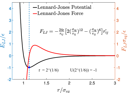
3. Integrate Newton's laws
Velocity Verlet Algorithm:
$$r(t+\Delta t)=r(t)+v(t) \Delta t+\frac{F_{LJ}(t)}{2 m} \Delta t^{2}$$$$r_{i}(t+\Delta t) = r_{i}(t) + v_{i}(t) + (a(t)/2) \Delta t^2 $$$$a(t+\Delta t) = F_{LJ}(r(t+\Delta t))/m$$$$v(t+\Delta t) = v(t) + 0.5 (a(t+\Delta t)+a(t))\Delta t $$Apply periodic boundary conditions (PBC)
Update $t$ to $t+\Delta t$
import MD
NSTEPS = 1000
row_col = [6,3] #row_col = [12,4]
lattice_spacing=[0.7,1.75]  # if hex
#lattice_spacing=[1.42,1.42]   # if bcc
sim = MD.Simulation(nSteps=NSTEPS, row_col=row_col, lattice="hex",  #"bcc""hex",
        lattice_spacing=lattice_spacing,
        print_frequency=100, dt=0.005, v_initial=2.5, temp=1.65,
        write_frequency=NSTEPS, store_frequency=10,traj_format="lammps")#"lammps")
# Verlet Algorithm
sim.integrate()